Using \(\mu\)sALEX #

The Problem #

\(\mu\)sALEX presents some issues for analysis with H²MM. The alternation period creates an artificial periodicity in the data. When using only the donor excitation streams, this results in gaps in photon arrivals, which does not materially impare anlaysis.

However, when incorporating the acceptor excitation stream, the alternation period results in periods of time where only donor excitation photons and other periods with only acceptor excitation. This creates two apparent “states” within the photon data, with a very predictable transition rate. Thus, using multi-parameter H²MM with \(\mu\)sALEX data, without special adjustments, will not yield meaningful results.

The Work-Around #

However, there is a work-around. Since we know the alternation period, we can assign each acceptor photon to a given acceptor excitation period, and identify the adjacent donor excitation period. Then the time of those photons can be reassigned into the adjacent donor excitation period. This removes the apparent alternation between all-donor and all-acceptor periods that H²MM would otherwise see. But it also destroys information about the time of acceptor photon arrivals. Therefore mpH²MM analysis of \(\mu\)sALEX must be taken with a grain of salt.

The main concern is that artifacts will remain due to the alternation period. If transition rates are close to or faster than the alternation period, they may be an artifact of the alternation period. Further examination of the results would therefore be necessary

If you use the defaults, when you create a BurstData object of data obtained with \(\mu\)sALEX, burstH2MM automatically applies this shift, according

Summary #

\(\mu\)sALEX data can be analayzed with essentially not additional work with burstH2MM.
Such analysis must be examined for artifacts due to the shift in photons

Therefore for \(\mu\)sALEX data you have 2 options:

Risk mpH²MM analysis, and gain the information about photophysics
Resort to spH²MM and forgoe the extra information, but be safe from artifacts from the alternation period.

Example #

For the file you can download here: HairPin3_RT_400mM_NaCl_A_31_TA.hdf5 , the transition rates are much slower than the alternation period. We have verified that mpH²MM analysis with the photon shift does not introduce artifacts. So the code bellow looks fundamenally the same as for nsALEX data.

[1]:

import numpy as np
from matplotlib import pyplot as plt

import fretbursts as frb
import burstH2MM as bhm

filename = 'HairPin3_RT_400mM_NaCl_A_31_TA.hdf5'
# load the data into the data object frbdata
frbdata = frb.loader.photon_hdf5(filename)
# if the alternation period is correct, apply data
# plot the alternation histogram
# frb.bpl.plot_alternation_hist(frbdata) # commented so not displayed in notebook
frb.loader.alex_apply_period(frbdata)
# calcualte the background rate
frbdata.calc_bg(frb.bg.exp_fit, F_bg=1.7)
# plot bg parameters, to verify quality
# frb.dplot(frbdata, frb.hist_bg) # commented so not displayed in notebook
# now perform burst search
frbdata.burst_search(m=10, F=6)
# make sure to set the appropriate thresholds of ALL size
# parameters to the particulars of your experiment
frbdata_sel = frbdata.select_bursts(frb.select_bursts.size, th1=50)
# make BurstData object to get data into bursth2MM

 - Optimized (cython) burst search loaded.
 - Optimized (cython) photon counting loaded.
--------------------------------------------------------------
 You are running FRETBursts (version 0.7.1).

 If you use this software please cite the following paper:

   FRETBursts: An Open Source Toolkit for Analysis of Freely-Diffusing Single-Molecule FRET
   Ingargiola et al. (2016). http://dx.doi.org/10.1371/journal.pone.0160716

--------------------------------------------------------------
# Total photons (after ALEX selection):    19,363,110
#  D  photons in D+A excitation periods:    6,728,731
#  A  photons in D+A excitation periods:   12,634,379
# D+A photons in  D  excitation period:    11,185,665
# D+A photons in  A  excitation period:     8,177,445

 - Calculating BG rates ... get bg th arrays
Channel 0
[DONE]
 - Performing burst search (verbose=False) ...[DONE]
 - Calculating burst periods ...[DONE]
 - Counting D and A ph and calculating FRET ...
   - Applying background correction.
   [DONE Counting D/A]

[ ]:

bdata = bhm.BurstData(frbdata_sel)

bdata.models.calc_models()

Look at the ICL to select the best model.

[ ]:

bhm.ICL_plot(bdata.models)

And plot the model with transition rates.

[ ]:

fig, ax = plt.subplots(figsize=(5,5))
bhm.dwell_ES_scatter(bdata.models[3], ax=ax)
bhm.scatter_ES(bdata.models[3], ax=ax)
bhm.trans_arrow_ES(bdata.models[3], ax=ax);

[ ]:

bhm.plot_burstjoin(bdata.models[2], 'transitions')

spH²MM to avoid any artifacts #

Here is how this data can be analyzed without the A_exA_emstream: simply specify the photon streams in ph_streams so that they only include the D_exstreams.

Note that the E-S plots no longer work, as the A_exA_emstream is no longer present within the data.

[ ]:

spdata = bhm.BurstData(frbdata_sel, ph_streams=[frb.Ph_sel(Dex='Dem'), frb.Ph_sel(Dex='Aem')])

spdata.models.calc_models()

[ ]:

bhm.ICL_plot(spdata.models)

[ ]:

bhm.dwell_E_hist(spdata.models[1])
bhm.axline_E(spdata.models[1])

[ ]:

spdata.models[1].trans

`shift` methods #

burstH2MM provides 3 options for precisely how the A_exA_emphotons are redistributed:

‘even’: (default): The number of A_exA_emphotons in each A_experiod are counted, and redistribute to evenly span the adjacent D_ex period.
‘rand’: Assign each A_exA_emphoton a random time within the adjacent D_ex period.
‘shift’: Shift all A_exA_emphotons by the difference between the beginning of the D_experiod and the beginning A_experiod. This is computationally the simplest adjustment, and maintains the rate fluctuations in the A_exA_emstream, but the shift means that fluctuations in A_exA_emintensity are misalligned with the cooresponding flucutations in the intensities of the D_exD_emand D_exA_emstreams. Also, if the A_experiod is shorter or longer than the D_experiod, then A_exA_emphotons will either not cover the entire D_experiod or extend beyond the D_experiod.

The method used is assigned when you create a BurstData object, by specifying the Aex_shift keyword argument.

If Aex_shift is not specified

Note

It is also possible to specify the Aex_shift=False to prevent any shifting of A_exA_emphotons. For \(\mu\)sALEX data, this will result in detecting the alternation period, and thus is generally discouraged, but still incldued as an option in burstH2MM for completeness, and to allow demonstration of the phenomenon of detecting the alternation period.

[8]:

bdata_false = bhm.BurstData(frbdata_sel, Aex_shift=False) # no Aex shift applied, discouraged
bdata_even = bhm.BurstData(frbdata_sel, Aex_shift='even') # distribute Aex photons evenly, default
bdata_rand = bhm.BurstData(frbdata_sel, Aex_shift='rand') # distribute Aex photons randomly
bdata_shift = bhm.BurstData(frbdata_sel, Aex_shift='shift') # shift by difference in start Dex and Aex periods

All subsequent data anlysis can be conducted as normal. Just be aware that since there are no nanotimes, you cannot access any lifetime based parameters or create divisors.

`shift` methods comparison #

Some comments about each method:

‘even’: There are no fluctuations in A_exA_em photon rate within a given alternation period, only between alternation periods. This reduces the chance of artifacts, but also means that these photons are no longer have poisson-distributed inter-photon times. This is the prefered method.
‘rand’: This keeps the poission distributed inter-photon times, but means that:
1. Each time a new BurstData object is created with Aex_shift='rand' , the photon times will be different
2. The random number generator could introduce other unexpected artifacts
‘shift’: This is computationally the simplest adjustment, and maintains the rate fluctuations in the A_exA_emstream, but it is generally discouraged for 2 key reasions:
1. The shift means that fluctuations in A_exA_emintensity are misalligned with the cooresponding flucutations in the intensities of the D_exD_emand D_exA_emstreams.
2. Also, if the A_experiod is shorter or longer than the D_experiod, then A_exA_emphotons will either not cover the entire D_experiod or extend beyond the D_experiod.

The are summarized in the table below:

Name	Method	Advantages	Disadvantages
‘even’	evenly distribute A_exA_em photons into the adjacent D_ex period	No rate fluctuations in the A_exA_em stream during a given alternation period	Even distribution of photons is not stochastic like all other photon times
‘rand’	Randomly distribute A_exA_em photons into the adjacent D_ex period	Maintains stochastic behavior of photon arrivals	Different each time, and randomness means potential for unpredictable artifacts in data
‘shift’	Shift A_exA_em streams by difference between start of D_ex and A_ex periods	Retains the most information from the A_exA_em stream	Realligned D_ex and A_ex rates, ‘overhangs’ when D_ex and A_ex periods are of different durations

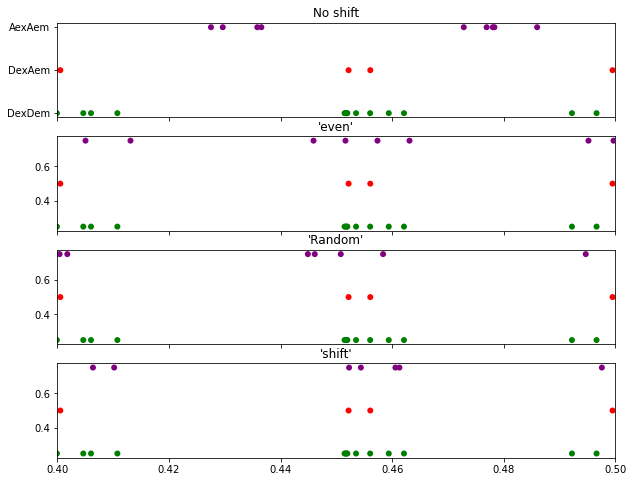
Bellow we have some code that plots the new photon times created by each of these methods:

[16]:

fig, ax = plt.subplots(4,1, figsize=(10,8), sharex=True)
n = 15
stream_color = {frb.Ph_sel(Dex='Dem'):'g', frb.Ph_sel(Dex='Aem'):'r', frb.Ph_sel(Aex='Aem'):'purple'}
bhm.plot_burst_index(bdata_false.models, n, ax=ax[0], stream_color=stream_color, stream_labels=True)
ax[0].set_title('No shift')
bhm.plot_burst_index(bdata_even.models, n, ax=ax[1], stream_color=stream_color)
ax[1].set_title("'even'")
bhm.plot_burst_index(bdata_rand.models, n, ax=ax[2], stream_color=stream_color)
ax[2].set_title("'Random'")
bhm.plot_burst_index(bdata_shift.models, n, ax=ax[3], stream_color=stream_color)
ax[3].set_title("'shift'")

ax[0].set_xlim([0.4, 0.5])

[16]:

(0.4, 0.5)

In summary, nsALEX data is always prefered, but if you check your transition rates and are careful, \(\mu\)sALEX analsysis is possible, and involves very little overhead with burstH2MM.

Download this documentation as a jupyter notebook here: usALEX.ipynb