Accessing the Results of an Optimization#
We start with some basic, universal loading and setup. This is the same in all how-tos and tutorials, so that there is a unified set of data to work with.
Note
Download the example file here: HP3_TE300_SPC630.hdf5
First let’s import the necessary modules and process the data with FRETBursts. This code is essential the same as that found in the tutorial .
[1]:
import numpy as np
from matplotlib import pyplot as plt

import fretbursts as frb
import burstH2MM as bhm

filename = 'HP3_TE300_SPC630.hdf5'
# load the data into the data object frbdata
frbdata = frb.loader.photon_hdf5(filename)
# plot the alternation histogram
# frb.bpl.plot_alternation_hist(frbdata) # commented so plot will not be displayed
# if the alternation period is correct, apply data
frb.loader.alex_apply_period(frbdata)
# calcualte the background rate
frbdata.calc_bg(frb.bg.exp_fit, F_bg=1.7)
# plot bg parameters, to verify quality
# frb.dplot(frbdata, frb.hist_bg) # commented so plot will not be displayed
# now perform burst search
frbdata.burst_search(m=10, F=6)
# make sure to set the appropriate thresholds of ALL size
# parameters to the particulars of your experiment
frbdata_sel = frbdata.select_bursts(frb.select_bursts.size, th1=50)
# frb.alex_jointplot(frbdata_sel) # commented so plot will not be displayed
 - Optimized (cython) burst search loaded.
 - Optimized (cython) photon counting loaded.
--------------------------------------------------------------
 You are running FRETBursts (version 0.7.1).

 If you use this software please cite the following paper:

   FRETBursts: An Open Source Toolkit for Analysis of Freely-Diffusing Single-Molecule FRET
   Ingargiola et al. (2016). http://dx.doi.org/10.1371/journal.pone.0160716

--------------------------------------------------------------
# Total photons (after ALEX selection):    11,414,157
#  D  photons in D+A excitation periods:    5,208,392
#  A  photons in D+A excitation periods:    6,205,765
# D+A photons in  D  excitation period:     6,611,308
# D+A photons in  A  excitation period:     4,802,849

 - Calculating BG rates ... get bg th arrays
Channel 0
[DONE]
 - Performing burst search (verbose=False) ...[DONE]
 - Calculating burst periods ...[DONE]
 - Counting D and A ph and calculating FRET ...
   - Applying background correction.
   [DONE Counting D/A]
Order of object creation#
Now that we’re done with FRETBursts to select our data, we can segment the photons into bursts, which will be stored in a BurstData object:
[2]:
bdata = bhm.BurstData(frbdata_sel)
H2MM_list.calc_models() is designed to streamline this process, which optimizes models until the ideal model is found (it actually calculates one more than necessary because it must see that there is at least one model with too many models).
So before H2MM_list.calc_models() is called on an H2MM_list object, it has no optimizations associated with it.
[3]:
try:
    bdata.models[0]
except Exception as e:
    print(e)
else:
    print('bdata has models')
No optimizations run, must run calc_models or optimize for H2MM_result objects to exist
After H2MM_list.calc_models() is called, then several different state models are stored in the H2MM_list.opts attribute, but are also accessible by indexing H2MM_list .
[4]:
# calculate models
bdata.models.calc_models()

bdata.models[0]
The model converged after 1 iterations
The model converged after 36 iterations
The model converged after 121 iterations
The model converged after 404 iterations
[4]:
| E_raw | S_raw | to_state_0 | |
|---|---|---|---|
| state_0 | 0.161329 | 0.687172 | 20000000.000000 |
The elements within H2MM_list are, as you see above, H2MM_result objects.
These serve to organize both the optimized models, and various results we will discuss later in this section.
But the first thing to examine are the statistical discriminators.
These take the loglikelihood of the model given the data, and add penalties for the number of states.
There are 2 primary discriminators:
BIC: the Bayes Information Criterion
Based on the likelihood of the model over all possible state paths through the data, usually found to always improve with more states, and therefore less useful
ICL: the Integrated Complete Likelihood
Based on the likelihood of the most likely state path through the data. Usually is minimized for the ideal state-model, and therefore the preferred statistical discriminator to use.
In both cases, the smaller the better.
Since these are computed for each optimized model, each H2MM_result object (index of H2MM_list ), has an attribute to get this value.
However, since these values are generally only useful in relation to other models optimized against the same data, the H2MM_result object has its own attribute to return an array with the values of all the optimized models:
BIC: H2MM_list.BIC : an array for every model in the list
[5]:
bdata.models.BIC
[5]:
array([323390.78889963, 274041.04580956, 266584.73431315, 265800.67189548])
and the value of for an individual model H2MM_result.bic
[6]:
bdata.models[0].bic
[6]:
323390.7888996289
ICL: H2MM_list.ICL : an array for every model in the list
[7]:
bdata.models.ICL
[7]:
array([323390.78889956, 275340.11281888, 269885.74586401, 271100.67269904])
and the value of for an individual model H2MM_result.icl
[8]:
bdata.models[0].icl
[8]:
323390.78889956296
burstH2MM has an easy, graphical way to compare these:
[9]:
# give ICL_plot a H2MM_list object
bhm.ICL_plot(bdata.models);
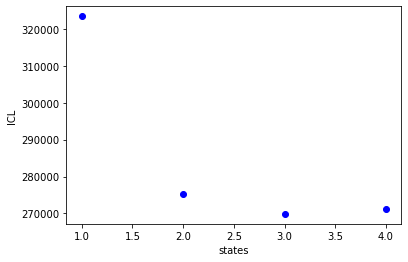
Note that we do not index bdata.models because this is comparing the different state models, not looking at a single model.
So now that we know how to select the model, what actually composes a model, which is stored in a H2MM_result object?
There are three key components:
Initial probability matrix (the .prior matrix) - The likelihood of a burst beginning in a given state
Observation probability matrix (the .obs matrix) - Contains probability a given state will emit a photon in a given index, from this the E and S values can be calculated.
Transition probability matrix (the .trans matrix) - The rate at which each state transitions to the others. This indicates the rate of transitions, characterizing the thermodynamic stability of each state (assuming you are using a model that has an appropriate number of states, over and underfit models will obviously have transition rates not reflective of the actual dynamics).
Note
The attribute names for the statistical discriminators from H2MM_list objects use capital letters, while H2MM_result objects are use lowercase letters.
The initial probability matrix does not have a clear physical meaning, but the observation probability and transition probability matrices contain very valuable information. burstH2MM automatically converts the values in these from the abstract units of the core algorithm into more human-friendly units (E/S values and transition rates in seconds).
E and S can be accessed with the attributes H2MM_result.E :
[10]:
bdata.models[2].E
[10]:
array([0.66031034, 0.15955158, 0.06730048])
and H2MM_result.S
[11]:
bdata.models[2].S
[11]:
array([0.43073408, 0.55348988, 0.9708039 ])
The above values are the raw values, if you want to have them corrected for leakage, direct excitation, and the beta and gamma values, you can access them by adding “ _corr “ to the attribute name, to get H2MM_result.E_corr and H2MM_result.S_corr .
The transition rates are accessed through the H2MM_result.trans attributes.
[12]:
bdata.models[2].trans
[12]:
array([[1.99994147e+07, 5.31727338e+02, 5.35450105e+01],
       [2.05278771e+02, 1.99996914e+07, 1.03279278e+02],
       [7.90911127e+00, 1.16271189e+02, 1.99998758e+07]])
These are in s -1 and the organization is [from state, to state]. Notice that the diagonal is all very large values, this is because the diagonal represents the probability that the system remains in the same state from one time step to the next, as the time steps are in the clock rate of the acquisiation (typically 20 mHz, meaning 50 ns from one time step to the next) this is a very large number.
Now H2MM also contains the Viterbi algorithm, which takes the data and optimized model, and finds the most likely state of each photon. burstH2MM continues to perform analysis on this state path to produce a number of usefull parameters to help understand the data.
Table of Attributes#
Below is a list and description of the different possible parameters and their descriptions.
Attribute |
Description |
Type |
|---|---|---|
Number of photons in each state and TCSPC bin |
state stream nanotime array |
|
Counts per dwell of states present within bursts |
state burst array |
|
Bininary code specifying the state present within each burst |
burst array |
|
The location of transitions with bursts |
burst list |
|
Duration of each dwell (in ms) |
dwell array |
|
The state of each dwell |
dwell array |
|
Numerical indicator of location within the burst of each dwell array |
dwell array |
|
Number of photons in each stream and dwell |
stream dwell array |
|
Background corrected number of photons in each stream and dwell |
stream dwell array |
|
Raw FRET efficiency (Eraw) of each dwell |
dwell array |
|
Fully corrected FRET efficiency of each dwell (E) |
dwell array |
|
Raw stoichiometry (Sraw) of each dwell |
dwell array |
|
Fully corrected stoichiometry of each dwell (S) |
dwell array |
|
Mean nanotime of each stream in each dwell |
stream dwell array |
Meaning of “type” explained in next section.
Understanding dwell array organization#
Data in dwell attributes (those that begin with “dwell”) are organized into numpy arrays.
As diagrammed in the figure below, the dwells are placed in the same order that they in the data.
This means the consecutive dwells indicate a transition from one state to another.
However, when one bursts ends, it is generally unreasonable to consider the dwell in the next burst to be considered a transition.
Hence, special consideration needs to be given for bursts at the start and end of bursts, as well as for bursts which contain only a single state, which is still counted as a dwell.
Since these are still included in the dwell arrays, the position of a burst within a dwell is recorded in the H2MM_result.dwell_pos paremeter.
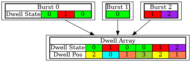
As seen, dwells in the middle of burst are marked with a 0 in H2MM_result.dwell_pos , end with a 1 , beginning with a 2 and bursts that span the whole dwell are marked with a 3 .
The size of H2MM_result.dwell_pos and other dwell array parameters match, and therefore H2MM_result.dwell_pos can be used to make masks to select only dwells in one of the possible positions.
For instance if you want to get the E values of only dwells that are in the middle of bursts, excluding beginning, ending and whole burst dwells, you could execute the following:
[13]:
mid_dwell_mask = bdata.models[2].dwell_pos == 0
mid_dwell_E = bdata.models[2].dwell_E[mid_dwell_mask]
print("Middle dwells:")
mid_dwell_E
Middle dwells:
[13]:
array([0.8       , 0.21875   , 0.55555556, 0.28571429, 0.58823529,
       0.27272727, 0.11111111, 0.85714286, 0.21428571, 0.08108108,
       0.66666667, 0.08571429, 0.58333333, 0.14285714, 0.        ,
       0.        , 0.2       , 0.70588235, 0.        , 0.74193548,
       0.08      , 0.06      , 0.57142857, 0.04651163, 0.63636364,
       0.775     , 0.85714286, 0.07692308, 0.57142857, 0.17021277,
       0.54166667, 1.        , 0.64285714, 0.03846154, 0.7       ,
       0.10526316, 0.        , 0.        , 0.23076923, 0.08108108,
       0.18181818, 0.5       , 0.83333333, 0.70454545, 0.2       ,
       0.07843137, 0.13333333, 0.71428571, 0.06666667, 0.77777778,
       0.875     , 0.14285714, 0.        , 0.76470588, 0.        ,
       0.9       , 0.56      , 0.72      , 0.08108108, 0.35714286,
       0.6       , 0.65909091, 0.13333333, 0.8       , 0.        ,
       0.55555556, 0.16853933, 0.75      , 0.24637681, 0.8       ,
       0.15      , 0.05660377, 0.6875    , 0.8125    ,        nan,
       0.54166667, 0.07692308, 0.        , 0.86666667, 0.14285714,
       0.075     , 0.10447761, 0.10606061, 0.17647059, 0.85714286,
       0.12      , 0.6       , 0.11111111, 0.71052632, 0.14634146,
       0.62857143, 0.06451613, 0.12121212, 0.16666667, 0.61111111,
       0.17647059, 0.71428571, 0.17647059, 0.24637681, 0.7       ,
       0.        , 0.5625    , 0.13636364, 0.22222222, 0.2       ,
       0.75      , 0.        , 0.07692308, 0.69230769, 0.        ,
       0.58333333, 0.5       , 0.16470588, 0.83333333, 0.128     ,
       0.10714286, 0.73076923, 0.08474576, 1.        , 0.76190476,
       0.07142857, 0.88888889, 0.6       , 0.        , 0.11111111,
       0.73076923, 0.22727273, 0.69230769, 0.        , 0.25490196,
       0.67741935, 0.77777778, 0.18518519, 0.        , 0.44444444,
       0.5862069 , 0.30612245, 0.04761905, 0.8       , 0.26785714,
       1.        , 0.28125   , 0.66666667, 0.75      , 0.16666667,
       0.78571429, 0.08      , 0.33333333, 0.1038961 , 0.11428571,
       0.76666667, 0.78431373, 0.56666667, 0.        , 0.6       ,
       0.51111111, 0.15      , 0.03846154, 1.        , 0.08108108,
       0.53846154, 0.22352941, 0.18181818, 0.8       , 0.05555556,
       0.22222222, 0.        , 0.06666667, 0.12121212, 0.11764706,
       0.125     , 0.57142857, 0.        , 0.73333333, 0.02564103,
       0.75      , 0.78947368, 0.20588235, 0.875     , 0.27272727,
       0.73333333, 0.16      , 0.04347826, 0.19587629, 0.06      ,
       0.81818182, 0.21052632, 0.85714286, 0.03921569, 0.33333333,
       0.33333333, 0.05769231, 0.        , 0.72727273, 0.11111111,
       0.78947368, 0.75      , 0.06666667, 0.375     ,        nan,
       0.02816901, 0.15909091, 0.57894737, 0.        , 0.14035088,
       0.51162791, 0.83333333, 0.11111111, 0.6       , 0.07142857,
       0.        , 0.51351351, 0.33333333, 0.08695652, 0.78571429,
       0.66666667, 0.69230769, 0.13513514, 0.09090909, 0.        ,
       0.5       , 0.28      , 0.13636364, 0.16666667, 0.05263158,
       0.02631579, 0.61764706, 0.6       , 0.57894737, 0.        ,
       1.        , 0.8       , 0.82608696, 0.13636364, 0.71428571,
       0.11111111, 0.44444444, 0.        , 0.66666667, 0.13513514,
       0.12727273, 0.25925926, 0.1       , 0.875     , 0.875     ,
       0.16666667, 0.15555556, 0.66666667, 0.125     , 0.        ,
       0.        , 0.8       , 0.05128205, 0.        , 0.0625    ,
       0.06896552, 0.77777778, 0.73076923, 0.05555556])
Now some of the dwell parameters have extra dimensions, like H2MM_result.dwell_nano_mean , where the mean nanotime is calculate per stream in addition to per dwell.
Therefore, it is a 2D array, with the last dimension marking the dwell.
Now, to get an accurate H2MM_result.dwell_nano_mean , we first need to set the IRF thresholds:
[14]:
bdata.irf_thresh = np.array([2355, 2305, 220])
So, with the BurstData.irf_thresh set, to get the mean nanotimes of the mid-burst dwells, we would execute the following:
[15]:
mid_dwell_mask = bdata.models[2].dwell_pos == 0
mid_dwell_nano_mean = bdata.models[2].dwell_nano_mean[:, mid_dwell_mask]

mid_dwell_nano_mean
[15]:
array([[ 5.28919324,  3.02778298,  3.07976408,  4.42869837,  1.83839165,
         2.11497928,  2.99796568,         nan,  2.2720322 ,  3.53096402,
         3.91131565,  5.02676288,  0.80131888,  4.31401096,  2.71656024,
         4.09526792,  3.82860111,  2.19385475,  2.07353476,  2.01958418,
         4.18760187,  3.45690921,  3.24925035,  3.75190694,  3.62486858,
         3.02259003,  4.32826206,  2.81541278,  2.1645382 ,  3.94518814,
         3.23703513,         nan,  1.00572035,  3.84502028,  7.40649924,
         4.2236496 ,  3.95926042,  4.24145992,  3.148314  ,  3.20631198,
         3.42922136,  1.453612  ,  1.36810541,  1.66432466,  3.38972546,
         3.73029762,  3.80175446,  2.98606774,  4.77411784,  1.61851756,
                nan,  2.4286092 ,  4.32317238,  4.07988578,  4.724239  ,
         0.36645681,  0.95957393,  3.37954611,  3.56204741,  4.53795679,
         1.80785358,  2.04944362,  2.21095607,  0.5008243 ,  3.34856546,
         4.11653146,  3.58945354,  2.53313268,  3.03955562,  2.3147855 ,
         3.02449018,  3.74143462,  3.74702085,  2.02162005,         nan,
         1.69028202,  2.77063555,  8.87436233,  0.89171156,  3.71885796,
         3.91430159,  4.06329151,  3.84734405,  2.78851705,  0.3175959 ,
         3.85334885,  0.72767852,  2.98307204,  0.45196339,  3.07300208,
         2.42472254,  3.71538341,  2.84207612,  3.01148969,  2.3605926 ,
         2.592447  ,  0.26873499,  4.07988578,  3.65185426,  5.38691506,
         1.41696632,  2.29820769,  2.92961858,  3.71702169,  2.78470157,
         2.4063997 ,  3.87752019,  3.49860947,  1.88419875,  1.91168301,
         5.57380803,  0.46417862,  4.65004946, 10.34629717,  3.52616955,
         2.72677178,  4.95716117,  3.92036929,         nan,  1.01691764,
         2.8442686 ,  1.42918155,  6.87717274,  3.85512561,  3.78512705,
         0.93324333,  4.78022546,  1.16655417,  4.51596938,  2.91909022,
         1.05923467,  7.51236454,  3.37780107,  3.53630818,  2.20790226,
         2.41128579,  2.31710218,  3.39111843,         nan,  4.08865569,
                nan,  4.30082206,  1.01793557,  0.92835724,  3.45012297,
         4.29975986,  4.99195606,  3.27368081,  4.25879187,  4.35156928,
         1.18313198,  2.84614787,  3.43247876,  1.91473681,  3.07212956,
         2.20790226,  2.93491185,  3.54880103,         nan,  4.01198349,
         2.89908051,  3.77882742,  2.48672407,  0.54561347,  3.76725232,
         4.7700461 ,  4.03102487,  3.53070954,  3.42343044,  5.23563417,
         4.52207699,  2.21872939,  3.84016195,  0.50693192,  3.90344361,
         2.54687481,  2.59369984,  2.68522553,         nan,  2.19686157,
         0.43567643,  3.66224136,  4.23096885,  3.46778578,  4.00768022,
         0.76345168,  4.1994205 ,  2.12544948,  3.63443717,  5.86941652,
         4.29823296,  3.0740788 ,  2.87835165,  7.53068738,  3.71081143,
         4.28449083,  1.0444019 ,  6.46098251,  3.82641982,         nan,
         3.80881553,  1.76347159,  2.75377021,  3.12961298,  3.82038007,
         3.03368752,  0.17101318,  3.36609165,  5.86330891,  3.11830312,
         4.98483051,  2.89644586,  6.21755049,  4.04581173,  0.51711127,
         6.28677011,  0.44585578,  2.14246354,  3.26553732,  4.32785489,
         0.72069839,  5.00824302,  2.26307437,  5.75031806,  3.13795606,
         4.31095716,  2.28813409,  1.39100896,  3.75170335,  5.06372051,
                nan,  0.94668008,  3.15763615,  4.14706953,  2.12370445,
         3.33475694,  6.50460832,  4.28088179,  5.07746264,  2.0586729 ,
         2.8485378 ,  2.15502319,  3.28436913,         nan,  0.12215227,
         1.49297218,  3.7520555 ,  3.21464054,  4.59964368,  3.4258159 ,
         2.92351097,  0.57411566,  3.96366662,  3.27775255,  4.23526347,
         3.36804942,  6.44353218,  1.31680146,  3.12709808],
       [ 6.8588499 ,  5.54396798,  5.28104976,  0.92530344,  6.40444346,
         5.41338138,  7.69559294,  3.33475694,  2.38196924,  4.57663834,
         4.3877095 ,  3.302183  ,  6.44527722,  1.89336017,         nan,
                nan,  2.37586163,  6.09234441,         nan,  4.8446652 ,
         2.34837737,  2.56926939,  5.2693435 ,  8.21474008,  4.18371521,
         4.08314317,  3.56828334,  1.93611346,  4.9532745 ,  4.67690499,
         2.54828426,  3.88240628,  5.88638211,  0.09772182,  4.28958051,
         4.52574156,         nan,         nan,  4.29568812,  8.03761929,
         5.7228338 ,  4.52835911,  4.4952035 ,  5.43892828, 14.64605704,
         2.43693776,  4.19593044,  4.07729467,  4.73950803,  3.05206169,
         2.57392281,  3.33475694,         nan,  4.68759332,         nan,
         3.67067568,  5.11643503,  5.06117567,  0.72884187,  5.44554815,
         3.61774303,  5.47494893,  4.73950803,  4.9059405 ,         nan,
         5.80223277,  5.55548519,  5.00905737,  3.51870389,  6.0419566 ,
         8.83160904,  0.44789165,  3.34253027,  3.86102963,         nan,
         3.57702561,  1.91779062,         nan,  5.14167089,  5.34619763,
         4.60921228,  2.2862833 ,  4.15666721,  5.80494727,  3.97300255,
         3.81115079,  5.06422948,  6.28880598,  6.34768963,  2.93369032,
         5.91216981,  6.77334331,  5.76558709,  3.18003073,  6.07985157,
         1.39864348,  2.62138769,  4.24937205,  3.90200154,  7.22443419,
                nan,  4.36490774,  7.8747496 ,  2.95608491,  7.65759001,
         5.41134551,         nan,  6.3152723 ,  4.74525637,         nan,
         4.32593535,  5.06321155,  4.47513562,  1.22885182,  6.0877637 ,
         3.96180525,  4.89927034,  3.02204713,  4.7700461 ,  4.30434057,
         6.18090481,  5.79307135,  2.76878476,         nan,  7.08890334,
         5.8337352 ,  5.75581491,  7.69711984,         nan,  4.71883611,
         3.81987595,  5.92438504,  4.06034142,         nan,  5.29224705,
         4.64681602,  5.53838387,  2.65884772,  5.33805415,  4.40073907,
         5.31769544,  7.06175839,  4.23664786,  5.19757904,  4.84639127,
         4.60291959,  2.43083015,  2.78507173,  7.48269899,  6.89244177,
         3.85445932,  3.88256288,  5.24895485,         nan,  6.75705634,
         2.91222114,  5.28104976,  9.71110538,  2.99028754,  3.68899852,
         2.92990942,  5.51163895,  6.94741029,  4.42343904,  7.06650876,
         5.18841762,         nan,  3.62181477,  2.77692825,  3.79893556,
         4.64178622,  3.85919735,         nan,  5.91949895,  2.73621082,
         3.60145606,  5.25254756,  4.2264685 ,  5.22113698,  4.72240672,
         4.48434552,  4.07683197,  3.99437919,  3.61355153,  3.48541141,
         3.11488286,  5.2250633 ,  2.15232298,  4.75172326,  1.69791654,
         5.98546118,  1.45768374,         nan,  2.53924029,  4.57460247,
         5.43821901,  5.90266908,  0.29316545,  2.93979794,         nan,
         4.58071008,  5.4052379 ,  4.17594188,         nan,  5.35026938,
         5.09258626,  3.61448564, 11.89763099,  6.38449192,  1.85060687,
                nan,  6.32298718,  1.05050951,  4.97770496,  4.94161451,
         5.24643995,  5.96510246,  5.93660027,  1.39253587,         nan,
         2.42472254,  4.95938212,  6.46999851,  1.453612  ,  1.36810541,
         2.89500877,  4.72322106,  3.62894032,  4.30208657,         nan,
         4.04866909,  4.58071008,  4.32351169,  6.9219619 ,  4.61588994,
         5.32583892,  6.63592201,         nan,  4.69919778,  3.70854288,
         4.58071008,  9.84896294,  4.9960278 ,  1.85322442,  3.38768959,
         4.84333746,  4.09454405,  2.35420736,  2.02772766,         nan,
                nan,  5.57625107,  2.49190629,         nan,  2.80034076,
         2.63848901,  5.91216981,  4.79994126,  5.59457392],
       [ 4.11277293,  3.94991577,  3.37893968,  3.13524157,  5.32865782,
         4.02578978,  2.64052488,  2.07658857,  4.68453951,         nan,
         5.04582834,  3.85797583,  3.6355569 ,  4.76149544,  2.86447071,
                nan,  4.15026875,  4.47484478,  3.74763161,  4.71536165,
         2.05826573,         nan,  3.48541141,  4.70286235,  4.30098139,
         3.68390884,  4.86104954,  2.9182177 ,  4.44557914,  3.75507179,
         3.68946834,  2.36839677,  4.54057434,  1.97886676,  4.21968227,
         4.04647354,  3.33359359,         nan,  4.75715225,  3.01716104,
         4.69064713,  3.9115871 ,  2.49434933,  3.73785943,  2.55053937,
         6.67358562,  2.95404904,  5.42382064,  4.21049475,  3.00441472,
         4.17854723,  4.33466051,         nan,  6.65322691,  2.82375328,
         4.6784319 ,  4.12492943,  5.71184009,         nan,  4.18100071,
         3.55288599,  3.76086951,  3.80324682,  4.51023762,  4.65400144,
         4.10724789,  4.12392489,  3.83319778,  4.82135005,  5.45148126,
         2.79660833,  1.36403367,  3.79893556,  3.36325914,  3.04973498,
         5.35075799,         nan,  4.34862077,  3.48291582,  3.52964533,
         8.43461417,  5.64343482,  4.58071008,  3.51416809,  5.6570595 ,
                nan,  4.60061638,  3.6713075 ,  4.32627585,  4.09304064,
         2.88007905, 15.59884474,  0.58225915,  3.44537261,  4.65970188,
         2.97807232,  2.63604596,  4.07135817,  6.1035417 ,  4.2421738 ,
         2.38196924,  3.50228005,         nan,  4.01392356,  4.4659742 ,
         2.87179984,  9.25914198,  8.79496336,  4.15317714,  3.24619655,
         3.65545512,  5.73640627,  3.82162098,  2.42777634,  4.21444717,
         8.09258781,  3.82995836,  0.46417862,  1.28259882,  3.40397656,
         2.28424743,  8.53030011,  3.6055278 ,         nan,  4.22937689,
         4.28690173,  3.10615769,  3.51870389,         nan,  4.94411308,
         3.54627324,  3.12954113,  4.1776076 ,  7.48386234,  4.57296384,
         3.10140399,  5.02387851,  1.53911859,  6.19922765,  4.36981778,
         2.07658857,  3.42716779,  3.82511105,  8.42697965,  5.25814621,
         4.93058908, 11.18914783,  5.35026938,  6.03432208,  3.44425772,
         3.82071053,  4.94988138,  4.36897948,  2.44711712,  4.70474162,
         3.65693355,  2.37518301,  3.48948315,  2.41250731,  1.78342313,
         3.23189187,  4.97788459,  4.05704862,  4.43005562,         nan,
         6.42520934,  2.75249779,         nan,         nan,  5.57537856,
         2.69142166,  4.41754955,  5.32176718,  5.63636285,  4.62346338,
         2.30867788,  2.79395553,  4.27088751,  3.79649252,  2.97644362,
         4.85310964,  5.39607648,  1.71013176,  2.79030683,         nan,
         4.52166982,  4.02350781,  6.16461784,         nan,  4.3552236 ,
         6.34581037,  5.37714288,  3.46135111,  3.71037517,  4.27908794,
         5.65658968,  4.55976969,  6.58400729,  3.91123684,  8.65448825,
         0.48860908,  3.97370727,  4.26893096,  1.25206076,  6.47407025,
         3.4710037 ,  4.98457602,  2.84933445,  3.47455343,  4.98381257,
         4.00863029,  3.94943638,  2.32496485,         nan,  5.0268567 ,
         4.87509705,  3.06689447,  3.85785607,  3.10642616,  4.34404006,
         3.21472906,  3.77503621,  3.87397196,  3.52612883,         nan,
         6.22976571,  5.20900619,  5.23596975,  3.4900189 ,  4.31916052,
         5.53502468,  3.93493176,  4.90659489,  4.65535869,  4.12407616,
         5.26679866,  4.62941637,         nan,  3.48215401,  3.99597248,
         5.23422472,  5.2265902 ,  3.47645357,  2.04197876,  2.53465958,
         5.20368665,  5.5964062 ,  4.15046265,  4.24438417,         nan,
         5.9060622 ,  3.0873986 ,  4.71813139,  2.80339457,  4.01270203,
         2.84207612,  4.09491991,  4.48214584,  3.64353073]])
Of course, you probably want to look at just on photon stream’s nanomean, more often than not this will be the D exDemstream, which for this data is the 0th stream.
So to get this we would execute the following:
[16]:
mid_dwell_mask = bdata.models[2].dwell_pos == 0
mid_dwell_nano_mean_DD = bdata.models[2].dwell_nano_mean[0, mid_dwell_mask]
mid_dwell_nano_mean_DD
[16]:
array([ 5.28919324,  3.02778298,  3.07976408,  4.42869837,  1.83839165,
        2.11497928,  2.99796568,         nan,  2.2720322 ,  3.53096402,
        3.91131565,  5.02676288,  0.80131888,  4.31401096,  2.71656024,
        4.09526792,  3.82860111,  2.19385475,  2.07353476,  2.01958418,
        4.18760187,  3.45690921,  3.24925035,  3.75190694,  3.62486858,
        3.02259003,  4.32826206,  2.81541278,  2.1645382 ,  3.94518814,
        3.23703513,         nan,  1.00572035,  3.84502028,  7.40649924,
        4.2236496 ,  3.95926042,  4.24145992,  3.148314  ,  3.20631198,
        3.42922136,  1.453612  ,  1.36810541,  1.66432466,  3.38972546,
        3.73029762,  3.80175446,  2.98606774,  4.77411784,  1.61851756,
               nan,  2.4286092 ,  4.32317238,  4.07988578,  4.724239  ,
        0.36645681,  0.95957393,  3.37954611,  3.56204741,  4.53795679,
        1.80785358,  2.04944362,  2.21095607,  0.5008243 ,  3.34856546,
        4.11653146,  3.58945354,  2.53313268,  3.03955562,  2.3147855 ,
        3.02449018,  3.74143462,  3.74702085,  2.02162005,         nan,
        1.69028202,  2.77063555,  8.87436233,  0.89171156,  3.71885796,
        3.91430159,  4.06329151,  3.84734405,  2.78851705,  0.3175959 ,
        3.85334885,  0.72767852,  2.98307204,  0.45196339,  3.07300208,
        2.42472254,  3.71538341,  2.84207612,  3.01148969,  2.3605926 ,
        2.592447  ,  0.26873499,  4.07988578,  3.65185426,  5.38691506,
        1.41696632,  2.29820769,  2.92961858,  3.71702169,  2.78470157,
        2.4063997 ,  3.87752019,  3.49860947,  1.88419875,  1.91168301,
        5.57380803,  0.46417862,  4.65004946, 10.34629717,  3.52616955,
        2.72677178,  4.95716117,  3.92036929,         nan,  1.01691764,
        2.8442686 ,  1.42918155,  6.87717274,  3.85512561,  3.78512705,
        0.93324333,  4.78022546,  1.16655417,  4.51596938,  2.91909022,
        1.05923467,  7.51236454,  3.37780107,  3.53630818,  2.20790226,
        2.41128579,  2.31710218,  3.39111843,         nan,  4.08865569,
               nan,  4.30082206,  1.01793557,  0.92835724,  3.45012297,
        4.29975986,  4.99195606,  3.27368081,  4.25879187,  4.35156928,
        1.18313198,  2.84614787,  3.43247876,  1.91473681,  3.07212956,
        2.20790226,  2.93491185,  3.54880103,         nan,  4.01198349,
        2.89908051,  3.77882742,  2.48672407,  0.54561347,  3.76725232,
        4.7700461 ,  4.03102487,  3.53070954,  3.42343044,  5.23563417,
        4.52207699,  2.21872939,  3.84016195,  0.50693192,  3.90344361,
        2.54687481,  2.59369984,  2.68522553,         nan,  2.19686157,
        0.43567643,  3.66224136,  4.23096885,  3.46778578,  4.00768022,
        0.76345168,  4.1994205 ,  2.12544948,  3.63443717,  5.86941652,
        4.29823296,  3.0740788 ,  2.87835165,  7.53068738,  3.71081143,
        4.28449083,  1.0444019 ,  6.46098251,  3.82641982,         nan,
        3.80881553,  1.76347159,  2.75377021,  3.12961298,  3.82038007,
        3.03368752,  0.17101318,  3.36609165,  5.86330891,  3.11830312,
        4.98483051,  2.89644586,  6.21755049,  4.04581173,  0.51711127,
        6.28677011,  0.44585578,  2.14246354,  3.26553732,  4.32785489,
        0.72069839,  5.00824302,  2.26307437,  5.75031806,  3.13795606,
        4.31095716,  2.28813409,  1.39100896,  3.75170335,  5.06372051,
               nan,  0.94668008,  3.15763615,  4.14706953,  2.12370445,
        3.33475694,  6.50460832,  4.28088179,  5.07746264,  2.0586729 ,
        2.8485378 ,  2.15502319,  3.28436913,         nan,  0.12215227,
        1.49297218,  3.7520555 ,  3.21464054,  4.59964368,  3.4258159 ,
        2.92351097,  0.57411566,  3.96366662,  3.27775255,  4.23526347,
        3.36804942,  6.44353218,  1.31680146,  3.12709808])
You could also isolate a particular state using the H2MM_result.dwell_state parameter to make another mask:
[17]:
mid_dwell_mask = bdata.models[2].dwell_pos == 0
state1_mask = bdata.models[2].dwell_state == 1
comb_mask = mid_dwell_mask * state1_mask
state1_mid_nano_mean_DD = bdata.models[2].dwell_nano_mean[0, comb_mask]
state1_mid_nano_mean_DD
[17]:
array([3.02778298, 4.42869837, 2.11497928, 2.99796568, 2.2720322 ,
       5.02676288, 4.31401096, 3.82860111, 2.07353476, 2.81541278,
       3.94518814, 4.2236496 , 3.95926042, 3.148314  , 3.42922136,
       3.38972546, 3.80175446, 4.77411784, 2.4286092 , 4.724239  ,
       4.53795679, 2.21095607, 3.34856546, 3.58945354, 3.03955562,
       3.02449018,        nan, 8.87436233, 3.71885796, 3.84734405,
       2.78851705, 2.98307204, 3.07300208, 3.01148969, 2.592447  ,
       4.07988578, 1.41696632, 3.71702169, 2.78470157, 1.91168301,
       4.65004946, 3.52616955, 2.72677178, 2.8442686 , 3.78512705,
       4.78022546, 2.91909022, 3.37780107, 3.53630818, 2.31710218,
       4.08865569, 4.30082206, 3.45012297, 3.27368081, 4.35156928,
       1.91473681, 2.93491185, 3.77882742, 2.48672407, 4.7700461 ,
       4.03102487, 5.23563417, 4.52207699, 3.84016195, 2.68522553,
       2.19686157, 3.66224136, 4.1994205 , 4.29823296, 2.87835165,
       3.71081143, 6.46098251,        nan, 1.76347159, 3.36609165,
       4.98483051, 6.21755049, 2.14246354, 3.26553732, 4.32785489,
       5.00824302, 2.26307437, 5.75031806, 5.06372051, 4.14706953,
       3.33475694, 2.0586729 , 2.15502319, 3.28436913, 1.49297218,
       3.7520555 , 4.59964368, 2.92351097, 3.27775255, 3.12709808])
Thus you can have a great deal of customization.
Example: Calculate variance of state 1 dwell E values#
Let’s put this into practice. Let’s say you want to know how tightly a given state’s dwell cluster around a given value. The steps would be simple:
Make mask of dwells in that state
Get E values of those dwells using mask
Calculate standard deviation (or whatever other value is of interest)
So lets see this in code:
[18]:
# make mask of dwells in state 1
state1_mask = bdata.models[2].dwell_state == 1
# get E values
state1_E = bdata.models[2].dwell_E[state1_mask]
# calculate standard deviation
np.nanstd(state1_E)
[18]:
0.12135964925716479
Note
We used np.nanstd, as dwells with no D exDemor DexAemphotons will have nan values, so we must exclude them to get a result that is not nan
Using masking functions to make masks#
burstH2MM also provides a set of masking functions in the Masking module.
They are named descriptively, and simply take a H2MM_list object as input.
So we can get the mid dwell mask like this:
[19]:
mid_dwell_mask = bhm.mid_dwell(bdata.models[2])
mid_dwell_mask
[19]:
array([False, False, True, ..., False, False, False])
These functions can be used to filter which dwells are shown in various plotting functions, which is their primary use in burstH2MM. See Plotting only dwells of certain position and other masking for a demonstration of thier use in plotting.
Burst Based Arrays#
In the list of attributes, you will notice two burst as opposed to dwell based attributes H2MM_result.burst_state_counts and H2MM_result.burst_type
These arrays are based not on dwells, but on the bursts instead.
H2MM_result.burst_state_counts is the larger, but ironically easier to understand of these arrays.
Going down the rows, you go through different states, each element indicating the number of dwells in that state, each column a different state.
[20]:
bdata.models[2].burst_state_counts
[20]:
array([[0, 2, 0, ..., 0, 0, 0],
       [0, 3, 0, ..., 0, 0, 1],
       [1, 0, 1, ..., 1, 1, 1]])
So for instance, the H2MM_result.burst_state_counts [1,23] will tell you how many dwells there were in state 1 burst 23.
H2MM_result.burst_type is essentially a simplification of H2MM_result.burst_state_counts where it no longer matters how many dwells in a given state are present, just whether there is at least one instance of a given state.
It represents this in a binary form, so a burst with only State0 will take the value 0b1 , while only State1 will have 0b10 , and a dwell with transitions between State0 and State1 will be represented as 0b11 .
Of course, python usually doesn’t display things in binary, so these will become 1, 2 and 3 when acutally displayed.
[21]:
bdata.models[2].burst_type
[21]:
array([4, 3, 4, ..., 4, 4, 6])
That’s the end of this How-To, thank you for using burstH2MM.
Download this documentation as a jupyter notebook here: ResultsAccess.ipynb