Discussion

What is H²MM?

H²MM is an extension of hiddenm Markov modeling, a broad set of methods for finding underlying behavior in noisy systems. The basic assumptions of hidden Markov models are:

1. The system is described by a Markvov model

   1. The data describes a system that transitions between a set of states.

   2. When the system is in a given state, it has a distinct set of probabilities to transition to each of the other states

   3. The system is memoryless, that is the probability to transition to another state is only influenced by the current state, and not any of the previous states

2. The model is hidden, meaning

   1. The states cannot be directly observed, rather

   2. Each state has a certain probability to produce certain observable results, with each state having a different set of probabilities

The earliest applications of HMM were towards language processing, for which it was not very successful, but has found much greater use in signal processing. HMM has also found extensive use in analyzing TIRF based smFRET trajectories. All of these applications however, assume that there is a constant data rate, for a camera with a set frame rate so that there is an image every ms.

This is not the case for single molecule confocal based data using single photon detectors. Here, data comes in sparsely, as individual photons, with varying interphoton times. H²MM extends the HMM algorithm to accept these variable interphoton times, allowing application of the HMM machinery with confocal data without implementing an external time bin.

HMM methods use the Baum-Welch algorithm in an optimization process which finds the model of a set number of states that best describes the data. Now since the number of states is fixed, other optimizations must be conducted with different numbers of states. Then the different optimized models must be compared, and the best one chosen, and the ones with too many (overfit) and too few (underfit) states rejected.

A final thing to understand about H²MM, is the use of indices. In H²MM, data comes in a set of detector chanels, in the first iterations, these were exclusively the D_exD_em and D_exA_em channels, but with mp H²MM, this was extended to the A_exA_em channel, and was even suggested to be able to include the parallel and perpendicular channels in anisotropy based measurements. A comparison to the original application of HMM methods is apt here: originally HMM was developed to analyze word patterns, so each word was a unique index, and each state had a given probability to produce each word. So in H²MM each photon can be compared to a word, each photon receives a set of a limited number of indices.

A Brief History of H²MM

Application to confocal single molecule data started with Gopich and Szabo 2009 who established the maximum likelihood estimator to calculated the likelihood of a model of transition rates and emission probabilities for a set of data. Pirchi and Tsukanov et. al. 2016 then integrated the Baum-Welch algorithm, with some reformulation of Gopich and Szabo’s original equations, which allowed for an optimization procedure ensuring that the likelihood of each iteration improves. This made finding the ideal model a feasible undertaking. However, discrimination between over and underfit models (models with too many or too few states), Lerner et. al. 2018 introduced the first attempt at this, with the modified Bayes Information Criterion, and finally the Integrated Complete Likelihood was introduced in Harris et. al. 2022, which proved a more reliable statistical discriminator. Harris et. al. 2022 also introduced the multiparameter approach, where the A_exA_em stream was integrated allowing discrimination of photophysical and FRET dynamics. They also introduced the H2MM_C python package, one which burstH2MM depends, which accelerated the calculations by implementing the core algorithm in C rather than in matlab, performing approximately 100 times faster.

Data organization

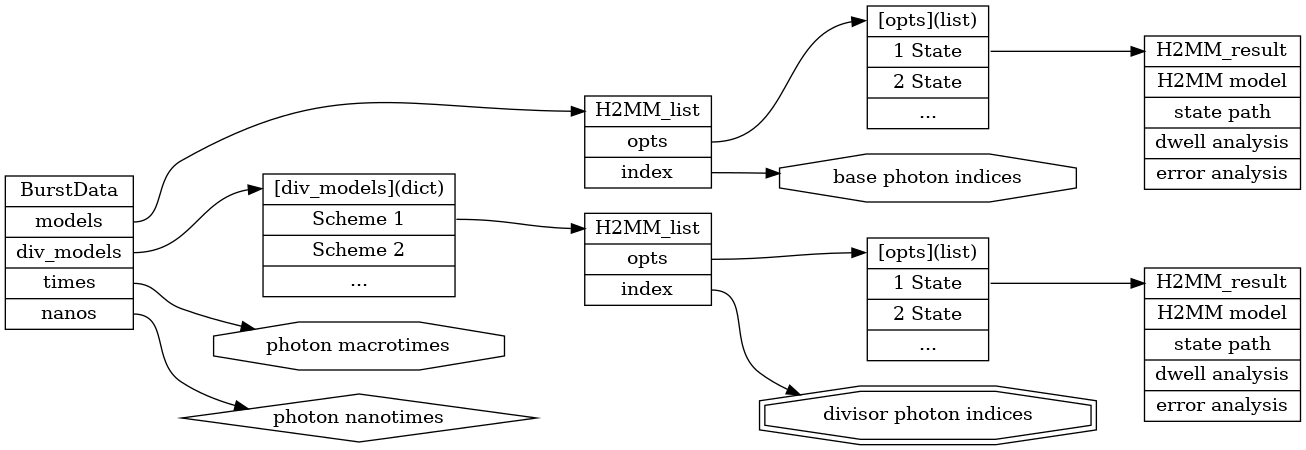
Map of data class reference in burstH2MM

In burstH2MM, there data analysis and organization is hierarchical. At the top there is the starting fretbursts.Data object, where the raw data is stored, and where the bursts are identified. The next level is the BurstData object, which serves 3 key roles:

1. Transition from fretbursts to burstH2MM

2. Select which set of photon streams to use (i.e. single vs multiparameter H²MM, excluding or including the A_exA_em stream)

3. Organize divisor schemes

Stored within the BurstData, in the BurstData.models attribute, is a H2MM_list object. This is created when the BurstData object is created.

The H2MM_list object serves primarily to:

1. Organize optimized models (Primary function)

2. Hold divisor schemes (Secondary function)

Underneath the H2MM_list object are H2MM_result objects, these

1. Hold an optimized model

2. Analyze Viterbi paths of optimized model

3. Generate dwell statistics

The BurstData object keeps track of all H2MM_list objects it creates, and likewise each H2MM_list object keeps track of all H2MM_result object that it creates.

For BurstData there are two places where the child H2MM_list objects are kept. The first is in the models attribute, the second is in the div_models attribute. models only has one H2MM_list associated with it, while div_models is a dictionary. models serves as the main model, which identifies photons only by photon stream (i.e. D_exD_em, D_exA_em, or A_exA_em), and as such serves as the main H²MM optimization. H2MM_list objects stored in div_models use divisor schemes to use photon nanotimes to further distinguish different photon streams.

On demand data creation

While burstH2MM is generally designed such that the user doesn’t have to interact directly with the times, and photon indexes, they are still accessible. Since the macrotime and nanotimes do not change, these are stored in the BurstData object, and H2MM_list objects reference their parent to get this data. However, the indexes, how H²MM identifies the photons, depends on the divisor scheme, and thus each H2MM_list object must have its own set of indexes.

Since all of these do not change from optimization to optimization, the H2MM_result object similarly uses reference to its parents to get this data. It is the state path and posterior probabilities that are unique to each individual optimization, so like the optimized model, these are also stored uniquely for each H2MM_result.

The rest of the calculated (mostly dwell based) parameters are similarly unique, and thus stored separately for each H2MM_result object. Here burstH2MM is designed to be smart in how it uses memory. With large data, each optimization creates a new set of data, which contains several values for each photon. This can eat up memory, so burstH2MM does not immediately calculate all these parameters once a model is optimized, rather it calculates the necessary arrays when the user requests said data. Therefore if certain parameters are never used, those arrays aren’t calculated. Thus many parameters aren’t calculated for non-ideal models. Because this does take time, once calculated burstH2MM keeps the calculated parameter in memory, so that future access does not require recalculating that parameter. If memory does become an issue, the method H2MM_result.trim_data() can be called, which clears all Viterbi based parameters, leaving only the optimized H²MM model still in memory. If a parameter is needed again, it can be recalculated without having to re-run the optimization.

Below the map of dependencies for each of the dwell parameters. To know what needs to be calculated for a given parameter, follow the arrows backwards to see which parameters will be calculated in order to access the given parameter.

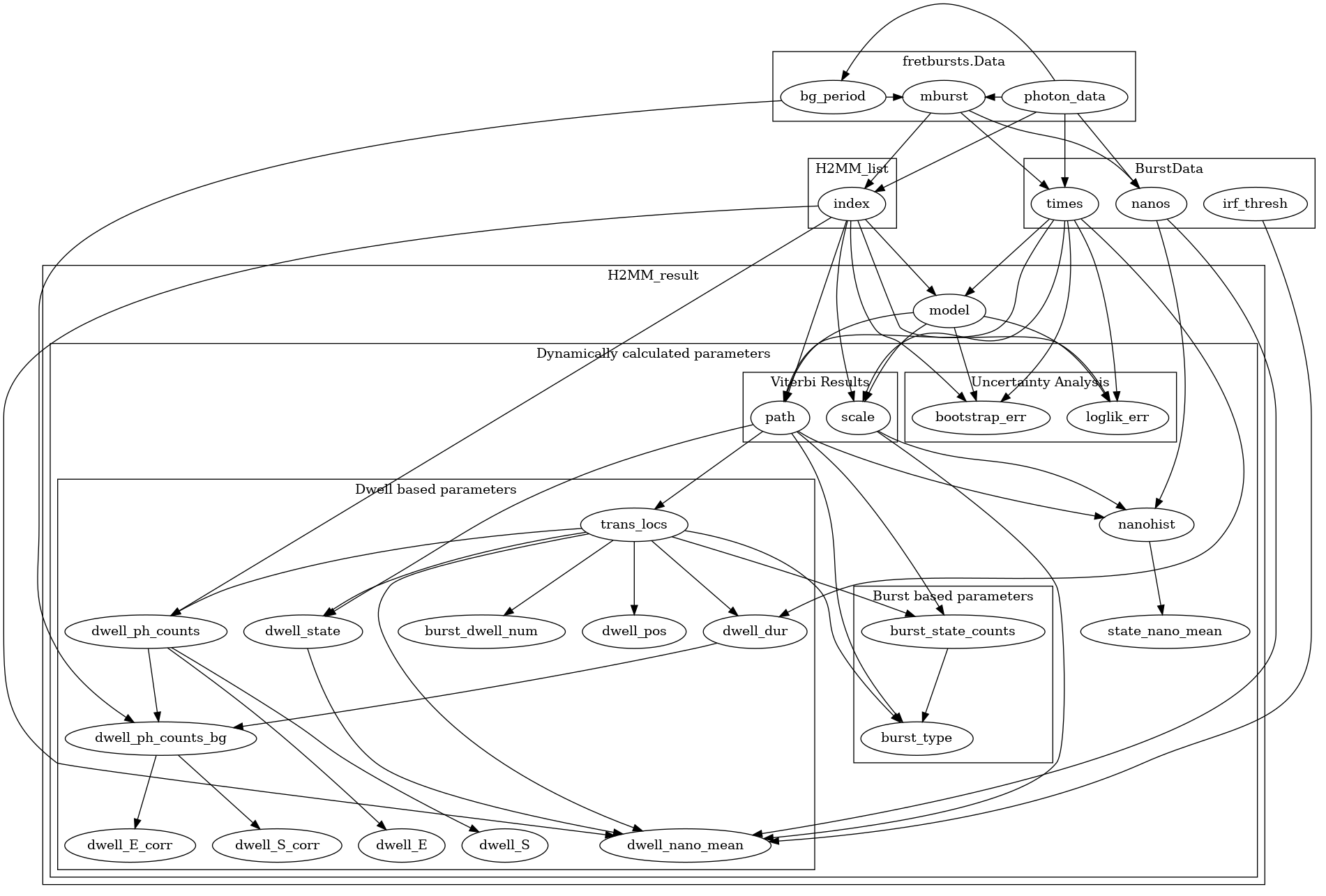
Parameters generation tree. Boxes indicate categories, if the name is that of a burstH2MM object, then all parameters within are attributes of said object.

Divisors

Note

This section is closely related with the how to section Customizing Divisors. It will be useful to read them together.

A more recent development in H²MM is the integration of photon nanotimes into H²MM analysis. The basic version of mp H²MM assigned photon indices only using the detector and excitation stream. With divisors, each of these streams an now be broken up into more indices by divisors.

If each nanotime received its own index, there would be too many for H²MM to properly analyze, so instead we use divisors to separate each excitation window into several nanotime based indices, many fewer than the raw nanotime bins would, and therefore making the optimization tractable for mp H²MM.

BurstData.auto_div() uses our even-division strategy to automatically assign what are hopefully sensible divisors. This however assumes that the underlying states have an at least somewhat equal population, and have a decay that is dominated by one exponential lifetime. If however you know that your system does not follow this pattern, you may want to consider BurstData.new_div() to use what you do know about your system to make a more sensible set of divisors.