Simulations #

Note

Download the example file here: HP3_TE300_SPC630.hdf5

First, let’s run the following code to generate a basic analysis for us to begin working with. This code is essential the same as that found in the tutorial .

[1]:

import numpy as np
from matplotlib import pyplot as plt

import fretbursts as frb
import burstH2MM as bhm

filename = 'HP3_TE300_SPC630.hdf5'
# load the data into the data object frbdata
frbdata = frb.loader.photon_hdf5(filename)
# if the alternation period is correct, apply data
# plot the alternation histogram
# frb.bpl.plot_alternation_hist(frbdata) # commented so not displayed in notebook
frb.loader.alex_apply_period(frbdata)
# calcualte the background rate
frbdata.calc_bg(frb.bg.exp_fit, F_bg=1.7)
# plot bg parameters, to verify quality
# frb.dplot(frbdata, frb.hist_bg) # commented so not displayed in notebook
# now perform burst search
frbdata.burst_search(m=10, F=6)
# make sure to set the appropriate thresholds of ALL size
# parameters to the particulars of your experiment
frbdata_sel = frbdata.select_bursts(frb.select_bursts.size, th1=50)
# make BurstData object to get data into bursth2MM
bdata = bhm.BurstData(frbdata_sel)
# calculate models
bdata.models.calc_models()
# set irf_thresh since later in tutorial we will discuss nanotimes
bdata.irf_thresh = np.array([2355, 2305, 220])

 - Optimized (cython) burst search loaded.
 - Optimized (cython) photon counting loaded.
--------------------------------------------------------------
 You are running FRETBursts (version 0.7.1).

 If you use this software please cite the following paper:

   FRETBursts: An Open Source Toolkit for Analysis of Freely-Diffusing Single-Molecule FRET
   Ingargiola et al. (2016). http://dx.doi.org/10.1371/journal.pone.0160716

--------------------------------------------------------------
# Total photons (after ALEX selection):    11,414,157
#  D  photons in D+A excitation periods:    5,208,392
#  A  photons in D+A excitation periods:    6,205,765
# D+A photons in  D  excitation period:     6,611,308
# D+A photons in  A  excitation period:     4,802,849

 - Calculating BG rates ... get bg th arrays
Channel 0
[DONE]
 - Performing burst search (verbose=False) ...[DONE]
 - Calculating burst periods ...[DONE]
 - Counting D and A ph and calculating FRET ...
   - Applying background correction.
   [DONE Counting D/A]

The model converged after 1 iterations

The model converged after 36 iterations

The model converged after 128 iterations

The model converged after 410 iterations

After an optimization has been conducted, several models are generated and compared. While statistical discriminators like the ICL and BIC are perhaps the most useful, another method to “check” the reasonableness of a model is to run a Monte-Carlo simulations. Using the probabilities derived from the model, and a set of arrival times, the sim.simulate() generates a set of photon indices (streams).

[2]:

sdata = bhm.sim.simulate(bdata.models[2])

The result is a special sim.Sim_Result object, which mimics a H2MM_result object, but uses the simulated times and stores the actual simulated path instead of the Viterbi path in the path variable.

Thus, you can interogate its parameters just like H2MM_result for instance:

[3]:

sdata.dwell_E

[3]:

array([0.08108108, 0.5       , 0.65625   , ..., 0.25      , 0.13793103,
       1.        ])

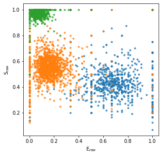
And it even functions in the plotting functions:

[4]:

fig, ax = plt.subplots(figsize=(5,5))
bhm.dwell_ES_scatter(sdata, ax=ax)

[4]:

[<matplotlib.collections.PathCollection at 0x7f2a0eb73f70>,
 <matplotlib.collections.PathCollection at 0x7f2a0e372550>,
 <matplotlib.collections.PathCollection at 0x7f2a0eb73f40>]

Note

The simulation does not simulate the photon nanotimes. While divisors are simulated, the individual nanotimes are not, and thus trying to access any nanotime-derived parameter in a sim.Sim_Result object will result in an error.

Download this documentation as a jupyter notebook here: Simulations.ipynb

Simulations#

Simulations #