Access Divisors and Models

We start with some basic, universal loading and setup. This is the same in all how-tos and tutorials, so that there is a unified set of data to work with.

Note

Download the example file here: HP3_TE300_SPC630.hdf5

First, let’s run the following code to generate a basic analysis for us to begin working with. This code is essentiall the same as that found in the tutorial .

import numpy as np
from matplotlib import pyplot as plt

import fretbursts as frb
import burstH2MM as bhm

filename = 'HP3_TE300_SPC630.hdf5'
# load the data into the data object frbdata
frbdata = frb.loader.photon_hdf5(filename)
# if the alternation period is correct, apply data
# plot the alternation histogram
# frb.bpl.plot_alternation_hist(frbdata) # commented so not displayed in notebook
frb.loader.alex_apply_period(frbdata)
# calcualte the background rate
frbdata.calc_bg(frb.bg.exp_fit, F_bg=1.7)
# plot bg parameters, to verify quality
# frb.dplot(frbdata, frb.hist_bg) # commented so not displayed in notebook
# now perform burst search
frbdata.burst_search(m=10, F=6)
# make sure to set the appropriate thresholds of ALL size
# parameters to the particulars of your experiment
frbdata_sel = frbdata.select_bursts(frb.select_bursts.size, th1=50)
bdata = bhm.BurstData(frbdata_sel)

 - Optimized (cython) burst search loaded.
 - Optimized (cython) photon counting loaded.
--------------------------------------------------------------
 You are running FRETBursts (version 0.7.1).

 If you use this software please cite the following paper:

   FRETBursts: An Open Source Toolkit for Analysis of Freely-Diffusing Single-Molecule FRET
   Ingargiola et al. (2016). http://dx.doi.org/10.1371/journal.pone.0160716

--------------------------------------------------------------
# Total photons (after ALEX selection):    11,414,157
#  D  photons in D+A excitation periods:    5,208,392
#  A  photons in D+A excitation periods:    6,205,765
# D+A photons in  D  excitation period:     6,611,308
# D+A photons in  A  excitation period:     4,802,849

 - Calculating BG rates ... get bg th arrays
Channel 0
[DONE]
 - Performing burst search (verbose=False) ...[DONE]
 - Calculating burst periods ...[DONE]
 - Counting D and A ph and calculating FRET ...
   - Applying background correction.
   [DONE Counting D/A]

Access within objects

In burstH2MM, whenever a new optimization result ( H2MM_result ) or divisor scheme ( H2MM_list ) is created, it is stored in a specific variable inside the creating object. Therefore, you can access such a result or divisor scheme through its parent. This also helps you keep track of which result belongs with which data set.

So, when we ran the optimization from the tutorial :

bdata.models.calc_models()

The model converged after 1 iterations

The model converged after 36 iterations

The model converged after 128 iterations

The model converged after 408 iterations

2

We were actually creating several H2MM_result objects. These can be referenced directly as indexes of the H2MM_list object

amodel = bdata.models[0]
type(amodel)

burstH2MM.BurstSort.H2MM_result

From these H2MM_result objects, we have access to the whole set of model- and dwell-based parameters of that particular optimization.

Note

Referencing an index under a H2MM_result object is identical to referencing an index of the attribute H2MM_list.opts H2MM_list.opts stores all the results in a list, and H2MM_list automatically treates indexing itself as indexing the list.

bdata.models[0] is bdata.models.opts[0]

True

When you run BurstData.auto_div() or BurstData.new_div() , a similar behavior occurs, where a new H2MM_result object is created, and placed inside the BurstData.div_models dictionary. So, looking at those results, you can access them by the key that was handed back.

Note that we use the name returned.

name = bdata.auto_div(2)
type(bdata.div_models[name])

burstH2MM.BurstSort.H2MM_list

Now, it can be annoying to constantly have to save the name of each new divisor, so burstH2MM offers an alternative: you can specify the name yourself before creating the divisor.

bdata.auto_div(2, name="mydivisor")
type(bdata.div_models["mydivisor"])

burstH2MM.BurstSort.H2MM_list

This can be useful if you have particular reasons for creating a certain divisor.

Examples of Object Refrencing and Creation

There are different ways to select/refer to the same objects. So, let’s see different examples of alternative ways to perform the same fundamental calculations.

Now, let’s see the code as it was before in the tutorial :

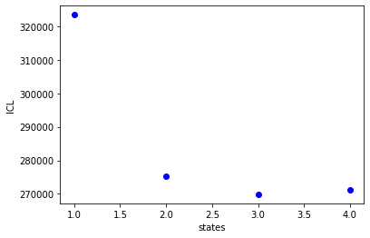
# calculate models
bdata.models.calc_models()
bhm.ICL_plot(bdata.models)

[<matplotlib.collections.PathCollection at 0x7fdd290f3910>]

Which we can re-write as:

models_list = bdata.models
models_list.calc_models()
bhm.ICL_plot(models_list)

[<matplotlib.collections.PathCollection at 0x7fdd290053d0>]

Finally, since these models are all connected, we can even swap the last lines like this:

models_list = bdata.models
models_list.calc_models()
# models_list refers to the same thing as bdata.models
bhm.ICL_plot(bdata.models)

[<matplotlib.collections.PathCollection at 0x7fdd28fe7d30>]

Now let’s look at this pattern with divisors, first we’ll initiate this code, and pull out the variables

bdata.auto_div(1, name="one_div")
# extract the H2MM_list divisor model into its own variable
div_list = bdata.div_models["one_div"]

So this:

bdata.div_models["one_div"].calc_models()

The model converged after 1 iterations

The model converged after 28 iterations

The model converged after 86 iterations

The model converged after 397 iterations

2

is the same as this:

div_list.calc_models()

2

That’s the end of this How-To, thank you for using burstH2MM.

Download this documentation as a jupyter notebook here: DivisorAccess.ipynb