Quantifying Accuracy/Precision of Model Parameter Values#
Note
Download the example file here: HP3_TE300_SPC630.hdf5
First, let’s run the following code to generate a basic analysis for us to begin working with. This code is essential the same as that found in the tutorial .
[1]:
import numpy as np
from matplotlib import pyplot as plt

import fretbursts as frb
import burstH2MM as bhm

filename = 'HP3_TE300_SPC630.hdf5'
# load the data into the data object frbdata
frbdata = frb.loader.photon_hdf5(filename)
# if the alternation period is correct, apply data
# plot the alternation histogram
# frb.bpl.plot_alternation_hist(frbdata) # commented so not displayed in notebook
frb.loader.alex_apply_period(frbdata)
# calcualte the background rate
frbdata.calc_bg(frb.bg.exp_fit, F_bg=1.7)
# plot bg parameters, to verify quality
# frb.dplot(frbdata, frb.hist_bg) # commented so not displayed in notebook
# now perform burst search
frbdata.burst_search(m=10, F=6)
# make sure to set the appropriate thresholds of ALL size
# parameters to the particulars of your experiment
frbdata_sel = frbdata.select_bursts(frb.select_bursts.size, th1=50)
# make BurstData object to get data into bursth2MM
bdata = bhm.BurstData(frbdata_sel)
# calculate models
bdata.models.calc_models()
 - Optimized (cython) burst search loaded.
 - Optimized (cython) photon counting loaded.
--------------------------------------------------------------
 You are running FRETBursts (version 0.7.1).

 If you use this software please cite the following paper:

   FRETBursts: An Open Source Toolkit for Analysis of Freely-Diffusing Single-Molecule FRET
   Ingargiola et al. (2016). http://dx.doi.org/10.1371/journal.pone.0160716

--------------------------------------------------------------
# Total photons (after ALEX selection):    11,414,157
#  D  photons in D+A excitation periods:    5,208,392
#  A  photons in D+A excitation periods:    6,205,765
# D+A photons in  D  excitation period:     6,611,308
# D+A photons in  A  excitation period:     4,802,849

 - Calculating BG rates ... get bg th arrays
Channel 0
[DONE]
 - Performing burst search (verbose=False) ...[DONE]
 - Calculating burst periods ...[DONE]
 - Counting D and A ph and calculating FRET ...
   - Applying background correction.
   [DONE Counting D/A]
The model converged after 1 iterations
The model converged after 36 iterations
The model converged after 128 iterations
The model converged after 414 iterations
[1]:
2
Bootstrap method#
Perhaps the easiest to understand method for quantifying uncertainty in a model is the bootstrap method. In this method, the bursts are split up into \(N\) subsets, and separate optimizations are run on each subset. Then the variance of each parameter value across the \(N\)different subsets serves as a quantification of the uncertainty.
In burstH2MM, the H2MM_result object has the H2MM_result.bootstrap_eval() method which performs this operation.
H2MM_result.bootstrap_eval() has one keyword argument: subsets by which you can specify the number of subsets to divide the data into.
The default is 10, which is usually a good compromise.
[2]:
bdata.models[2].bootstrap_eval(subsets=5)
The model converged after 290 iterations
The model converged after 226 iterations
The model converged after 2017 iterations
The model converged after 227 iterations
The model converged after 268 iterations
[2]:
(array([[89.31520909, 60.39327263, 51.39814368],
        [32.52744943, 36.89787477, 24.65788966],
        [ 8.20605449, 16.43892423, 12.39367234]]),
 array([0.0255139 , 0.00435775, 0.00127755]),
 array([0.00960336, 0.00264025, 0.00212474]))
Note how the number of subsets is the number of optimizations. This method automatically stores the results in the H2MM_result.bootstrap_err attribute, and the transition rate, E, and S values are also supplied as return values.
Once you run bootstrap_eval, you can now access trans_std_bs , E_std_bs , S_std_bs attributes of H2MM_result , which are the standard deviations of each parameter of the optimized models of the subsets.
[3]:
bdata.models[2].trans_std_bs
[3]:
array([[89.31520909, 60.39327263, 51.39814368],
       [32.52744943, 36.89787477, 24.65788966],
       [ 8.20605449, 16.43892423, 12.39367234]])
[4]:
bdata.models[2].E_std_bs, bdata.models[2].S_std_bs
[4]:
(array([0.0255139 , 0.00435775, 0.00127755]),
 array([0.00960336, 0.00264025, 0.00212474]))
Closer examination of models#
H2MM_result.bootstrap_err attribute allows closer examination of these subsets.
This attribute is an instance of the class ModelError.Bootstrap_Error , which is made to coordinate the bootstrap evaluation.
The H2MM_result attributes H2MM_result.trans_std_bs , H2MM_result.E_std_bs , H2MM_result.S_std_bs are just aliases of the attributes of ModelError.Bootstrap_Error.trans_std , ModelError.Bootstrap_Error.E_std , and ModelError.Bootstrap_Error.S_std in its H2MM_result.bootstrap_err attribute.
[5]:
bdata.models[2].bootstrap_err.trans_std
[5]:
array([[89.31520909, 60.39327263, 51.39814368],
       [32.52744943, 36.89787477, 24.65788966],
       [ 8.20605449, 16.43892423, 12.39367234]])
[6]:
bdata.models[2].bootstrap_err.E_std, bdata.models[2].bootstrap_err.S_std
[6]:
(array([0.0255139 , 0.00435775, 0.00127755]),
 array([0.00960336, 0.00264025, 0.00212474]))
For E and S, the leakage/direct excitation/ \(\gamma\)and \(\beta\)correct values: ModelError.Boostrap_Error.E_std_corr , and ModelError.Boostrap_Error.S_std_corr
[7]:
bdata.models[2].bootstrap_err.E_std_corr, bdata.models[2].bootstrap_err.S_std_corr
[7]:
(array([0.0255139 , 0.00435775, 0.00127755]),
 array([0.00960336, 0.00264025, 0.00212474]))
If on the other hand, you would prefer to take the standard error, instead of standard deviation of the subsets, there are equivalent attributes ModelError.Bootstrap_Error.trans_err , ModelError.Bootstrap_Error.E_err , and ModelError.Bootstrap_Error.S_err .
[8]:
bdata.models[2].bootstrap_err.trans_err
[8]:
array([[39.94297579, 27.0086926 , 22.98594864],
       [14.54671761, 16.50123124, 11.02734349],
       [ 3.66985913,  7.35171041,  5.54261877]])
[9]:
bdata.models[2].bootstrap_err.E_err, bdata.models[2].bootstrap_err.S_err
[9]:
(array([0.01141016, 0.00194885, 0.00057134]),
 array([0.00429475, 0.00118076, 0.00095021]))
For E and S, the leakage/direct excitation/ \(\gamma\)and \(\beta\)correct values: ModelError.Bootstrap_Error.E_err_corr , and ModelError.Bootstrap_Error.S_err_corr
[10]:
bdata.models[2].bootstrap_err.E_err_corr, bdata.models[2].bootstrap_err.S_err_corr
[10]:
(array([0.01141016, 0.00194885, 0.00057134]),
 array([0.00429475, 0.00118076, 0.00095021]))
You can also see the values of the individual subset models.
This is done through the attribute ModelError.Bootstrap_Error.models .
This attribute is again another special class, ModelError.ModelSet used for organizing models that vary only in their specific parameter values, but share the same number of states, and data and divisor scheme.
It lets you access the transition rate, E and S values as attributes, and for E and S, access these with the ModelError.ModelSet.trans , ModelError.ModelSet.E , ModelError.ModelSet.S attributes respectively. For E and S, the leakage/direct excitation/\(\gamma\)and \(\beta\)correct values are accessible with the ModelError.ModelSet.E_corr and ModelError.ModelSet.S_corr attributes.
The organization of these arrays is [state, subset] for E and S, and [from_state, to_state, subset] for transition rates.
[11]:
bdata.models[2].bootstrap_err.models.trans
[11]:
array([[[1.99993025e+07, 5.47412626e+02, 1.50107894e+02],
        [2.56911399e+02, 1.99996697e+07, 7.33960161e+01],
        [2.71844461e+01, 9.25543456e+01, 1.99998803e+07]],

       [[1.99994454e+07, 5.01289522e+02, 5.33486484e+01],
        [2.02533298e+02, 1.99996915e+07, 1.06001520e+02],
        [7.16681031e+00, 1.38306883e+02, 1.99998545e+07]],

       [[1.99994312e+07, 5.68807992e+02, 2.21385758e-05],
        [2.15768390e+02, 1.99996411e+07, 1.43089271e+02],
        [4.79837339e+00, 1.25242149e+02, 1.99998700e+07]],

       [[1.99995343e+07, 4.36098017e+02, 2.95648463e+01],
        [1.55146963e+02, 1.99997508e+07, 9.40438819e+01],
        [7.29023492e+00, 1.10009269e+02, 1.99998827e+07]],

       [[1.99993033e+07, 6.12696880e+02, 8.40199625e+01],
        [2.11897860e+02, 1.99997083e+07, 7.98318819e+01],
        [8.19442843e+00, 1.01374572e+02, 1.99998904e+07]]])
[12]:
bdata.models[2].bootstrap_err.models.E, bdata.models[2].bootstrap_err.models.S
[12]:
(array([[0.63874832, 0.16143698, 0.06563951],
        [0.66284056, 0.15296923, 0.06698833],
        [0.67054299, 0.15811327, 0.06875795],
        [0.62598318, 0.16620047, 0.06867949],
        [0.69909413, 0.15815619, 0.06616314]]),
 array([[0.43073864, 0.55001657, 0.97045621],
        [0.43598782, 0.55806882, 0.97225223],
        [0.43725447, 0.55429823, 0.9687245 ],
        [0.43685133, 0.55273276, 0.96839454],
        [0.4119258 , 0.55269972, 0.97400269]]))
[13]:
bdata.models[2].bootstrap_err.models.E_corr, bdata.models[2].bootstrap_err.models.S_corr
[13]:
(array([[0.63874832, 0.16143698, 0.06563951],
        [0.66284056, 0.15296923, 0.06698833],
        [0.67054299, 0.15811327, 0.06875795],
        [0.62598318, 0.16620047, 0.06867949],
        [0.69909413, 0.15815619, 0.06616314]]),
 array([[0.43073864, 0.55001657, 0.97045621],
        [0.43598782, 0.55806882, 0.97225223],
        [0.43725447, 0.55429823, 0.9687245 ],
        [0.43685133, 0.55273276, 0.96839454],
        [0.4119258 , 0.55269972, 0.97400269]]))
Loglikelihood Uncertainty Evaluation#
The bootstrap error is very simple, however, it also can take a long time, and the particular subsets used may have a significant influence on the calculated values.
What is loglikelihood uncertainty?#
The assessment of the loglikelihood uncertainties relies on finding the loglikelihood of models where one of the model parameter values has been offset from the optimal value. While a full statistical analysis would require integration across the whole parameter space, we note that the loglikelihoods generally distribute in a Gaussian-like manner, and therefore we can approximate the uncertainty by finding the point at which the loglikelihood is some amount less than the optimal model:
:math:` LL(lambda _{Delta E_{n}}) = LL(lambda _{optimal}) - 0.5`
There are two points at which this is true, one where \(E_{n}\)is greater than the optimal \(E_{n}\), and another, where \(E_{n}\)is less than the optimal \(E_{n}\), denoted \(E_{n, high}\)and \(E_{n, low}\)respectively.
The errors reported are thus:
\(err_{LL}(E) = \frac{E_{n,high} - E_{n,low}}{2}\)
Note that in most cases, \(E_{n, high} - E_{n, optimal} \approx E_{n, optimal} - E_{n, low}\)
This is not true however, for transition rates, and thus, in lieu of reporting an average value to represent a +/- type of error, instead we report directly the high and low transition rates.
Calculating loglikelihood uncertainty#
Estimation of Loglikelihood uncertainty is handled by ModelError.Loglik_Error objects, which are created automatically when a H2MM_result object is created, and stored in the H2MM_result.loglik_err attribute.
Upon its creation, no values are actually calculated, only the skeleton exists.
All parameter times (E/S/transition rates) follow the same basic rules, so we will start by demonstrating uncertainty estimation for E.
To estimate the uncertainty for E, we use the ModelError.Loglik_Error.get_E_err() method.
[14]:
E_err = bdata.models[2].loglik_err.get_E_err(0)
E_err
[14]:
0.005624999999999991
The equivalent for the stoichiometry is ModelError.Loglik_Error.get_S_err() :
[15]:
S_err = bdata.models[2].loglik_err.get_S_err(2)
S_err
[15]:
0.00077636718749996
These value indicate the point at which models where a given parameter value is varied from the optimal, have a loglikelihood 0.5 less than the optimal model, ie:
:math:` LL(lambda _{Delta E_{n}}) = LL(lambda _{optimal}) - 0.5`
There are two points at which this is true, one where \(E_{n}\)is greater than the optimal \(E_{n}\), and another, where \(E_{n}\)is less than the optimal \(E_{n}\), denoted \(E_{n, high}\)and \(E_{n, low}\)respectively.
The errors reported are thus:
\(err_{LL}(E) = \frac{E_{n,high} - E_{n,low}}{2}\)
Note that in most cases, \(E_{n, high} - E_{n, optimal} \approx E_{n, optimal} - E_{n, low}\)
This is not true however, for transition rates, and thus, in lieu of reporting an average value to represent a +/- type of error, instead we report directly the high and low transition rates.
[16]:
trans_err = bdata.models[2].loglik_err.get_trans_err(0,1)
trans_err
[16]:
masked_array(data=[501.8588059030635, 562.3571669228339],
             mask=[False, False],
       fill_value=inf)
The ModelError.Loglik_Error.get_E/S_err() methods also allow passing the keyword parameter simple as simple=False to return the low/high values like ModelError.Loglik_Error.get_trans_err()
[17]:
E_err = bdata.models[2].loglik_err.get_E_err(0, simple=False)
E_err
[17]:
masked_array(data=[0.6546853599116289, 0.6659353599116289],
             mask=[False, False],
       fill_value=nan)
[18]:
S_err = bdata.models[2].loglik_err.get_S_err(0, simple=False)
S_err
[18]:
masked_array(data=[0.4273356364488786, 0.43415204269887864],
             mask=[False, False],
       fill_value=nan)
Accessing Values Previously Calculated#
Calculations of the uncertainty values are stored in masked arrays, so that only calculated values are available.
These can be accessed through the attributes ModelError.Loglik_Error.E , ModelError.Loglik_Error.S , ModelError.Loglik_Error.trans .
[19]:
bdata.models[2].loglik_err.trans
[19]:
masked_array(
  data=[[[--, --],
         [501.8588059030635, 562.3571669228339],
         [--, --]],

        [[--, --],
         [--, --],
         [--, --]],

        [[--, --],
         [--, --],
         [--, --]]],
  mask=[[[ True,  True],
         [False, False],
         [ True,  True]],

        [[ True,  True],
         [ True,  True],
         [ True,  True]],

        [[ True,  True],
         [ True,  True],
         [ True,  True]]],
  fill_value=inf)
[20]:
bdata.models[2].loglik_err.E
[20]:
masked_array(data=[0.005624999999999991, --, --],
             mask=[False,  True,  True],
       fill_value=nan)
[21]:
bdata.models[2].loglik_err.S
[21]:
masked_array(data=[0.003408203125000009, --, 0.00077636718749996],
             mask=[False,  True, False],
       fill_value=nan)
The ModelError.Loglik_Error.E and ModelError.Loglik_Error.S are a little more processed than the ModelError.Loglik_Error.trans , as these do not show the low/high directly for a given state, but rather show half the difference between them.
If you want to see the actual low and high values, these can be accessed with the ModelError.Loglik_Error.E_lh and ModelError.Loglik_Error.S_lh attributes (this is basically the same as passing the simple=False keyword argument to ModelError.Loglik_Error.get_E_err() / ModelError.Loglik_Error.get_S_err() ):
[22]:
bdata.models[2].loglik_err.E_lh
[22]:
masked_array(
  data=[[0.6546853599116289, 0.6659353599116289],
        [--, --],
        [--, --]],
  mask=[[False, False],
        [ True,  True],
        [ True,  True]],
  fill_value=nan)
[23]:
bdata.models[2].loglik_err.S_lh
[23]:
masked_array(
  data=[[0.4273356364488786, 0.43415204269887864],
        [--, --],
        [0.9700226579124809, 0.9715753922874808]],
  mask=[[False, False],
        [ True,  True],
        [False, False]],
  fill_value=nan)
Concluding this list of access attributes, the loglikelihood values of these models are also stored in the ModelError.Loglik_Error.E_ll , ModelError.Loglik_Error.S_ll , and ModelError.Loglik_Error.trans_ll attributes:
[24]:
bdata.models[2].loglik_err.E_ll
[24]:
masked_array(
  data=[[-133208.37002081441, -133208.37125588267],
        [--, --],
        [--, --]],
  mask=[[False, False],
        [ True,  True],
        [ True,  True]],
  fill_value=-inf)
[25]:
bdata.models[2].loglik_err.S_ll
[25]:
masked_array(
  data=[[-133208.36515007372, -133208.36806724593],
        [--, --],
        [-133208.36725677058, -133208.36851899815]],
  mask=[[False, False],
        [ True,  True],
        [False, False]],
  fill_value=-inf)
Adjusting thresholds#
From the earlier equation, the estimated error is defined by having a loglikelihood \(0.5\)less than the optimal, however, if you wish to change this threshold, to say \(1.0\), this can be done (before running any get_ method) by setting the ModelError.Loglik_Error.thresh attribute:
[26]:
bdata.models[2].loglik_err.thresh = 1.0
S_err = bdata.models[2].loglik_err.get_S_err(1)
S_err
[26]:
0.00277343749999992
Another factor that can be adjusted is how precisely the search algorithm needs to find the loglikelihood, this factor is stored in the ModelError.Loglik_Error.flex attribute. The default is \(0.005\)
[27]:
bdata.models[2].loglik_err.flex = 5e-2
E_err = bdata.models[2].loglik_err.get_E_err(1)
E_err
[27]:
0.002695312500000005
These set univeral threshold/flex values, is generally preferred, these values can be altered for each calculation.
This works by passing thresh and flex keyword arguments to the ModelError.Loglik_Error.get_E_err() / ModelError.Loglik_Error.get_S_err() / ModelError.Loglik_Error.get_trans_err() .
Warning
Passing thresh and flex keyword arguments to the ModelError.Loglik_Error.get_E_err() / ModelError.Loglik_Error.get_S_err() / ModelError.Loglik_Error.get_trans_err() will only affect the current calculation.
Therefore all other calculations will have different thresh and flex values, and therefore will not be comparable to one another.
This is why it is discouraged to use this method.
[28]:
E_err = bdata.models[3].loglik_err.get_E_err(2, thresh=0.1, flex=1e-2)
E_err
[28]:
0.0010156249999999922
Clearing Values#
Since values already stored are not recalculated, if a new threshold is set, previous values can be cleared using the ModelError.Loglik_Error.clear_E ModelError.Loglik_Error.clear_S() , and ModelError.Loglik_Error.clear_trans() , and ModelError.Loglik_Error.clear_all() methods.
These reset their respective arrays:
[29]:
bdata.models[2].loglik_err.clear_E()
bdata.models[2].loglik_err.clear_S()
bdata.models[2].loglik_err.clear_trans()
As the name suggests, ModelError.Loglik_Error.clear_all() clears all the values.
So the three lines above, together do what is done bellow in a single line:
[30]:
bdata.models[2].loglik_err.clear_all()
Calculating All Uncertainty Values#
When a given H2MM_result has only a few states, it will not take long to characterize the uncertainty of all model parameters, but for 5+ states, this becomes time consuming.
Hence the choice to break with burstH2MM’s normal strategy of calculating on demand and storing the result, and instead using a ModelError.Loglik_Error.get_E_err / ModelError.Loglik_Error.get_S_err / ModelError.Loglik_Error.get_trans_err strategy, and masked arrays, that unmask values that have been calculated.
However, if you so desire, the ModelError.Loglik_Error.all_eval() method provides a shortcut, and evaluates all parameters for you.
This is great for 2 and 3 state models, workable for 4 state models, and less advisable for 5+ state models.
[31]:
# reset thresh and flex to default before re-calculating everything
bdata.models[2].loglik_err.thresh, bdata.models[2].loglik_err.flex = 0.5, 5e-3

# evaluate all parameters
bdata.models[2].loglik_err.all_eval()
bdata.models[2].loglik_err.trans
[31]:
masked_array(
  data=[[[--, --],
         [501.8588059030635, 562.3571669228339],
         [40.92595696232948, 67.31424834784906]],

        [[193.29419084215726, 217.69955433877388],
         [--, --],
         [95.36877509434665, 111.5681913319069]],

        [[3.735882210708648, 12.60135444968205],
         [108.29230392786711, 124.56154227875899],
         [--, --]]],
  mask=[[[ True,  True],
         [False, False],
         [False, False]],

        [[False, False],
         [ True,  True],
         [False, False]],

        [[False, False],
         [False, False],
         [ True,  True]]],
  fill_value=inf)
[32]:
bdata.models[2].loglik_err.E
[32]:
masked_array(data=[0.005624999999999991, 0.0019238281250000128,
                   0.0010351562500000022],
             mask=[False, False, False],
       fill_value=nan)
[33]:
bdata.models[2].loglik_err.S
[33]:
masked_array(data=[0.003408203125000009, 0.001953125, 0.00077636718749996],
             mask=[False, False, False],
       fill_value=-inf)
Examining Loglikelihood Variance Along a Given Parameter#
So far uncertainty estimation has been built finding how far a given parameter must be varied to alter the loglikelihood by a certain value.
This is done by an iterative process, and each iteration is saved.
The parameter values and loglikelihoods are stored in attributes of ModelError.Loglik_Error .
Parameter type |
Parameter Value |
Loglikelihood |
|---|---|---|
E |
||
S |
||
Trans |
These are 2D (for trans) and 1D (for E/S) numpy object arrays, whose elements are 1D numpy arrays of all values/loglikelihoods evaluates thus far.
These arrays however will often have values clustered around where the search value is, whereas for more in-depth analysis, it would be more convenient to have an evenly spaced set of values.
Such arrays can be generated by the ModelError.Loglik_Error.E_space() , ModelError.Loglik_Error.S_space() , and ModelError.Loglik_Error.trans_space() methods.
The only required argument to these functions is the state or transition for which to calculate the array.
The rng and steps keyword arguments let you specify the range over which to space the parameter values, and the number of values to evaluate (think of this as similar to the numpy linspace and logspace functions).
steps is always a positive integer.
rng however has several options:
Option |
Behavior |
When callable |
|
|---|---|---|---|
int/float |
multiply value by difference between low/high value and optimal value to offset for low/high values of range |
Must have evaluated uncertainty before calling |
No |
2 element array-like (tuple, list, numpy array) |
low/high values for the range |
Call anytime |
No |
Many element array-like |
The individual values of the specified parameter to evaluate the matrix, steps ignored |
Call anytime |
Yes |
Note
If rng is not specified, it behaves like rng=2 and therefore prior to evaluating, you must have already performed ModelError.Loglik_Error.get_E_err() / ModelError.Loglik_Error.get_S_err() / ModelError.Loglik_Error.get_trans_err() for the given state or transition.
[34]:
Erng, Ell = bdata.models[2].loglik_err.E_space(0)
Erng[0], Erng[-1], Erng.size
[34]:
(0.6490603599116289, 0.6715603599116289, 20)
[35]:
Srng, Sll = bdata.models[2].loglik_err.S_space(1, rng=3, steps=10)
Srng[0], Srng[-1], Srng.size
[35]:
(0.5476305043691996, 0.5593492543691996, 10)
Note
For ModelError.Loglik_Error.trans_space() the transition must be specified as a 2-tuple of (from_state, to_state).
[36]:
trng, tll = bdata.models[2].loglik_err.trans_space((0,1), rng=(100, 400))
trng[0], trng[-1], trng.shape
[36]:
(99.99999999999999, 400.0, (20,))
The return values of these ModelError.Loglik_Error.E_space() / ModelError.Loglik_Error.S_space() / ModelError.Loglik_Error.trans_space() methods are automatically added to the ModelError.Loglik_Error.E_rate_rng / ModelError.Loglik_Error.S_rate_rng / ModelError.Loglik_Error.t_rate_rng and ModelError.Loglik_Error.E_ll_rng / ModelError.Loglik_Error.S_ll_rng / ModelError.Loglik_Error.t_ll_rng attributes, and so we can access all previously calculated values.
Note that these are stored in arrays of arrays, so you must specify the state/(from_state, to_state) that you want to access.
[37]:
bdata.models[2].loglik_err.t_ll_rng[0,1]
[37]:
array([-133421.33099232, -133408.78806882, -133396.23640999,
       -133383.70003837, -133371.20575538, -133358.78339051,
       -133346.46606703, -133334.29048486, -133322.29722086,
       -133310.53104671, -133299.04126446, -133287.88205962,
       -133277.11287135, -133266.79877898, -133257.01090395,
       -133247.82682552, -133239.33100829, -133231.61523905,
       -133224.77906936, -133218.93026009, -133209.34821107,
       -133208.70964879, -133208.45556987, -133208.39896862,
       -133208.37171389, -133208.34515839, -133208.24595844,
       -133207.99849657, -133208.16408984, -133208.27247109,
       -133208.33312831, -133208.36508243, -133208.3981236 ])
Plotting Parameters#
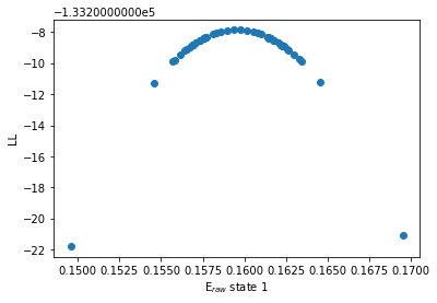
It is also possible to plot how the loglikelihood varies along a given parameter.
This uses the ll_E_scatter() , ll_S_scatter() and ll_trans_scatter() functions.
These functions take as required arguments a H2MM_result or ModelError.Loglik_Error object, and which state to plot. For ll_E_scatter() and ll_S_scatter , this is a single integer, indicating the index of the state. For ll_trans_scatter() this is two arguments: from_state and to_state .
[38]:
bhm.ll_E_scatter(bdata.models[2],1)
[38]:
<matplotlib.collections.PathCollection at 0x7f9e0103a880>

By default the ll_E_scatter() plots only an evenly spaced distribution of parameter values, it does this by calling ModelError.Loglik_Error.E_space() and plots only those values. You can pass the rng and steps keyword arguments to ll_E_scatter() , and these will be passed to ModelError.Loglik_Error.E_space() , to adjust the values plotted.
If on the other hand, you would like to see all values that have been evaluated, you can pass the keyword argument: rng_only=False , and it will plot all the values for the given parameter (everything stored in ModelError.Loglik_Error.E_rng )
[39]:
bhm.ll_E_scatter(bdata.models[2],1, rng_only=False)
[39]:
<matplotlib.collections.PathCollection at 0x7f9e007c6af0>
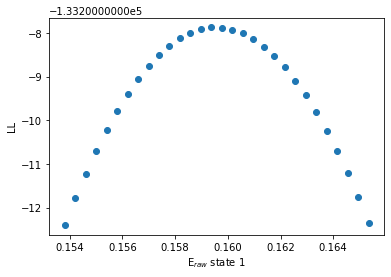
Now let’s see the same for the stoichiometry, same rules apply:
[40]:
bhm.ll_E_scatter(bdata.models[2],1, rng=3, steps=30)
[40]:
<matplotlib.collections.PathCollection at 0x7f9e039bb9d0>
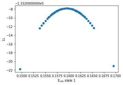
[41]:
bhm.ll_E_scatter(bdata.models[2],1, rng=3, steps=30, rng_only=False)
[41]:
<matplotlib.collections.PathCollection at 0x7f9e03aa6850>
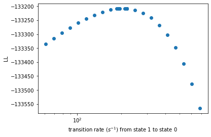
And for transition rates, note that ll_trans_scatter() needs two indices for from_state and to_state , instead of just one.
[42]:
bhm.ll_trans_scatter(bdata.models[2], 1,0)
[42]:
<matplotlib.collections.PathCollection at 0x7f9e039efeb0>

[43]:
bhm.ll_trans_scatter(bdata.models[2], 1,0, rng=1.5, rng_only=False)
[43]:
<matplotlib.collections.PathCollection at 0x7f9e00569310>
Forcing Recalculation#
The ModelError.Loglik_Error.get_E_err() / ModelError.Loglik_Error.get_S_err() / ModelError.Loglik_Error.get_trans_err() methods check if a value has been calculated, and can return such values without repeating the calculation.
There are however lower level methods that calculate values regardless of whether they were calculated before, and over-write the value if it was.
These are the ModelError.Loglik_Error.E_eval() , ModelError.Loglik_Error.S_eval() , and ModelError.Loglik_Error.trans_eval() methods.
Note
Unlike the ModelError.Loglik_Error.get_E/S/trans_err() methods, these methods do not have a return value, they just write their value to the corresponding array in the ModelError.Loglik_Error object.
If these methods are called with no keyword arguments, then all values of E, S, or trans will be calculated, but if only specific values are to be calculated, you can specify the locs keyword argument.
The locs keyword argument must be an iterable object where the elements are the desired states or transitions.
These methods also accept the same thresh and flex keyword arguments, and come with the same warnings of setting them individually instead of globally as for ModelError.Loglik_Error.get_E_err() / ModelError.Loglik_Error.get_S_err() / ModelError.Loglik_Error.get_trans_err() .
Also present is the max_iter keyword argument which specifies how many iterations of the search algorithm to execute seeking a loglikelihood close to thresh less than the optimal, within a range of flex .
Finally, for ModelError.Loglik_Error.E_eval() / ModelError.Loglik_Error.S_eval() , there is the step keyword argument, and for ModelError.Loglik_Error.trans_eval() there is the factor argument, which specify the offset from the optimal value to use as an initial value in the search algorithm.
[44]:
# clear previously stored values so re-evaluation can be tested
bdata.models[2].loglik_err.clear_all()

bdata.models[2].loglik_err.E_eval(locs=(0,1))
bdata.models[2].loglik_err.E
[44]:
masked_array(data=[0.005624999999999991, 0.0019238281250000128, --],
             mask=[False, False,  True],
       fill_value=nan)
[45]:
bdata.models[2].loglik_err.S_eval(locs=(0,1))
bdata.models[2].loglik_err.S
[45]:
masked_array(data=[0.003408203125000009, 0.001953125, --],
             mask=[False, False,  True],
       fill_value=-inf)
[46]:
bdata.models[2].loglik_err.trans_eval(locs=((0,1), (1,0),))
bdata.models[2].loglik_err.trans[:,:,0]
[46]:
masked_array(
  data=[[--, 501.8588059030635, --],
        [193.29419084215726, --, --],
        [--, --, --]],
  mask=[[ True, False,  True],
        [False,  True,  True],
        [ True,  True,  True]],
  fill_value=inf)
Covariant optimizations#
In the previous characterization of uncertainty, only a single parameter value could be varied at a time. Ideally we could make an N-dimensional grid of all combinations of parameter varied around their optimal values, but the shear number of points on such an N-dimensional grid grows so quickly with more states that such a method is not implemented here.
Instead, we can take one parameter at a time, fix it’s value to various offsets from the optimal, and find the optimal values for all other parameters. Thus we can see how changing one parameter affects the others, and how closely correlated they are to one another.
This is done through the covariance methods: ModelError.Loglik_Error.covar_trans() , ModelError.Loglik_Error.covar_E() and ModelError.Loglik_Error.covar_S() .
Similar to the ModelError.Loglik_Error.E_space / ModelError.Loglik_Error.S_space / ModelError.Loglik_Error.trans_space functions for the basic loglikelihood error, these functions take the particular transition/state you would like to evaluate as arguments, and also take the same rng and steps keyword arguments.
Note
Since these are optimization based parameters, these functions also take max_iter and converged_min keyword arguments to control when optimization terminates.
Once finished, the results are stored in the corresponding index of ModelError.Loglik_Error.trans_covar , ModelError.Loglik_Error.E_covar , and ModelError.Loglik_Error.S_covar , each of which is a numpy masked array of ModelError.ModelSet objects, so the calculated values will be stored in the corresponding index.
As with the ModelError.Bootstrap_Error.models attribute that was a ModelError.ModelSet object, access to the individual optimized parameters is provided through the appropriately named attributes.
[47]:
bdata.models[2].loglik_err.covar_E(0)
bdata.models[2].loglik_err.E_covar[0].E[:,1]
The model converged after 82 iterations
The model converged after 78 iterations
The model converged after 74 iterations
The model converged after 66 iterations
The model converged after 53 iterations
The model converged after 54 iterations
The model converged after 68 iterations
The model converged after 76 iterations
The model converged after 80 iterations
The model converged after 84 iterations
[47]:
array([0.15892296, 0.15906223, 0.15920173, 0.15934149, 0.15948151,
       0.15962176, 0.15976239, 0.15990334, 0.16004464, 0.16018629])
[48]:
bdata.models[2].loglik_err.covar_S(1)
bdata.models[2].loglik_err.S_covar[1].S[:,0]
The model converged after 52 iterations
The model converged after 50 iterations
The model converged after 47 iterations
The model converged after 43 iterations
The model converged after 34 iterations
The model converged after 34 iterations
The model converged after 44 iterations
The model converged after 50 iterations
The model converged after 57 iterations
The model converged after 59 iterations
[48]:
array([0.43215553, 0.43183874, 0.43152246, 0.43120671, 0.43089146,
       0.4305768 , 0.43026259, 0.4299489 , 0.42963572, 0.42932306])
[49]:
bdata.models[2].loglik_err.covar_trans(0,1)
bdata.models[2].loglik_err.trans_covar[0,1].trans[:,0,1]
The model converged after 76 iterations
The model converged after 77 iterations
The model converged after 80 iterations
The model converged after 83 iterations
The model converged after 80 iterations
The model converged after 92 iterations
The model converged after 136 iterations
The model converged after 211 iterations
Optimization reached maximum number of iterations
Optimization reached maximum number of iterations
[49]:
array([ 158.70168905,  207.5797375 ,  271.51158681,  355.13361109,
        464.51012722,  607.57318246,  794.6977911 , 1039.45433638,
       1359.59270244, 1778.329506  ])
Plotting Covariance#
There are 3 functions for plotting the results of covariance: covar_trans_ll_scatter() , covar_E_ll_scatter() and covar_S_ll_scatter() .
These plot the loglikelihood of the optimized models against the value of the fixed parameter, they take two arguments: the ModelError.Loglik_Error data, and the state to plot, or in the case of covar_ll_trans_scatter() , the particular transition, and thus 3 arguments are required, the ModelError.Loglik_Error data, from_state and to_state :
Note
This function is smart, and will take either the base H2MM_result or ModelError.Loglik_Error , if the former, it will automatically extract the ModelError.Loglik_Error object from the H2MM_result.loglik_err attribute.
Note
If you have not already run ModelError.Loglik_Error.covar_trans() / ModelError.Loglik_Error.covar_E() / ModelError.Loglik_Error.covar_S() for the given state/transition, these functions will automatically run these with default parameters.
[50]:
bhm.covar_trans_ll_scatter(bdata.models[2].loglik_err, 0,1)
[50]:
<matplotlib.collections.PathCollection at 0x7f9e004ccfd0>

These functions all also take the standard ax keyword argument, and all additional keyword arguments are passed to ax.scatter()
[51]:
fig, ax = plt.subplots()
bhm.covar_E_ll_scatter(bdata.models[2], 0, ax=ax, s=60, marker='+', c='r')
[51]:
<matplotlib.collections.PathCollection at 0x7f9e00459460>

Now there are a lot more values to plot, for instance, it is nice to see how when one parameter is offset, how does that affect the optimal values of other parameters. There are no built-in plotting functions for this, since specifying which parameter makes the function signatures rather long and awkward, so such plots are left to the user. Thankfully, if you know which particular combination of parameters you want to plot, it is not very difficult to setup your custom plots.
This will also be a good way to teach how to access these different values.
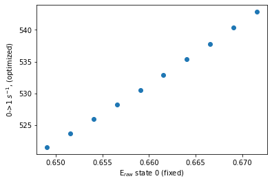
So say we want to see how, when the FRET efficiency of state 0 is varied, how does that affect the transitions from state 0 to state 1?
To do this we need to extract these parameters, and then plot them.
For demonstration purposes, we’ll do this in 3 steps
Isolate the covariance results (
ModelError.ModelSetobject) of state 0.Extract the (fixed) E values of state 0, and the (optimized) transition values from state 0 to state 1
Plot covariance
[52]:
# get the ModelSet of state 0 E_covar
covar_E_state0 = bdata.models[2].loglik_err.E_covar[0]

# get fixed E values for x and optimized
# note: we use ':' for the 0th dimension, so we look at each model
# then specify the state/transition of interest
x = covar_E_state0.E[:,0]
y = covar_E_state0.trans[:,0,1]

# plot
plt.scatter(x,y)

plt.xlabel("E$_{raw}$ state 0 (fixed)")
plt.ylabel(r"0->1 $s^{-1}$, (optimized)")
[52]:
Text(0, 0.5, '0->1 $s^{-1}$, (optimized)')
Of course, we could just do this all in one line (plus axis labels):
[53]:
plt.scatter(bdata.models[2].loglik_err.E_covar[0].E[:,0], bdata.models[2].loglik_err.E_covar[0].trans[:,0,1])
plt.xlabel("E$_{raw}$ state 0 (fixed)")
plt.ylabel(r"0->1 $s^{-1}$, (optimized)")
[53]:
Text(0, 0.5, '0->1 $s^{-1}$, (optimized)')

Of course, there is no need to restrict ourselves to having the x axis be the fixed parameter, we can see how they all vary with one another, and maybe we’ll give the fixed parameter as a color argument:
[54]:
x = bdata.models[2].loglik_err.E_covar[0].E[:,1] # state 1 E values
y = bdata.models[2].loglik_err.E_covar[0].E[:,2] # state 2 E values
c = bdata.models[2].loglik_err.E_covar[0].E[:,0] # state 0 E values (fixed)
c /= c.max() # normalize values since using cmap
plt.scatter(x, y, c=c, cmap='viridis')
plt.xlabel("E$_{raw}$ state 1 (optimized)")
plt.ylabel("E$_{raw}$ state 2 (optimized)")
[54]:
Text(0, 0.5, 'E$_{raw}$ state 2 (optimized)')

Finally, let’s think about combining the results of different covariances, we can use a 3-D plot to show how loglikelihood changes with respect to two parameters.
So we’ll take the covariance of E in state 0, and the covariance of S in state 1, plotting those values with E state 0 and S state 1 on the x and y axis, that way we can see the shape of two fixed axes with 1 free axis together.
[55]:
xE = bdata.models[2].loglik_err.E_covar[0].E[:,0] # state 0 E values
yE = bdata.models[2].loglik_err.E_covar[0].S[:,1] # state 1 E values
zE = bdata.models[2].loglik_err.E_covar[0].loglik # loglikelihood, note that there is no state specification

xS = bdata.models[2].loglik_err.S_covar[1].E[:,0] # state 0 E values
yS = bdata.models[2].loglik_err.S_covar[1].S[:,1] # state 1 E values
zS = bdata.models[2].loglik_err.S_covar[1].loglik # loglikelihood, note that there is no state specification

fig = plt.figure(figsize=(10,10))
ax = fig.add_subplot(projection='3d')

ax.scatter(xE, yE, zE, label='fixed: E$_{raw}$ state 0')
ax.scatter(xS, yS, zS, label='fixed: S$_{raw}$ state 1')

ax.set_xlabel("E$_{raw}$ state 0")
ax.set_ylabel("S$_{raw}$ state 1")
ax.set_zlabel("LL")
ax.legend()
[55]:
<matplotlib.legend.Legend at 0x7f9e001e8d90>
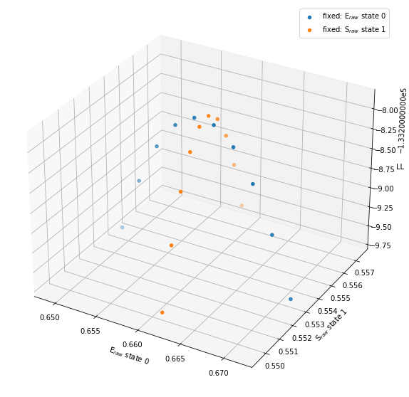
The key point, is that you have access to all non-lifetime model parameters (not dwell parameters) through identically named elements, and you can see how they correlate with one another and the overall logliklihood.
Download this documentation as a jupyter notebook here: Uncertainty.ipynb